线性代数的基本操作

标量由只有一个元素的张量表示

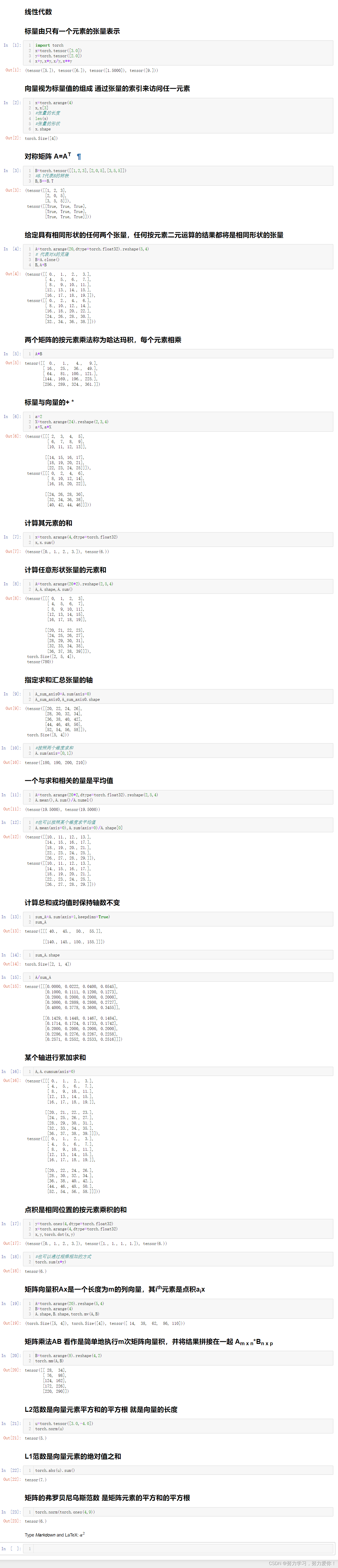
import torch
x=torch.tensor([3.0])
y=torch.tensor([2.0])
x+y,x*y,x/y,x**y

向量视为标量值的组成 通过张量的索引来访问任一元素

x=torch.arange(4)
x,x[3]
#张量的长度
len(x)
#张量的形状
x.shape

对称矩阵 A=AT

B=torch.tensor([[1,2,3],[2,0,5],[3,5,5]])
#B.T代表B的转秩
B,B==B.T

给定具有相同形状的任何两个张量，任何按元素二元运算的结果都将是相同形状的张量

A=torch.arange(20,dtype=torch.float32).reshape(5,4)
# 代表对A的克隆
B=A.clone()
B,A+B

两个矩阵的按元素乘法称为哈达玛积，每个元素相乘

A*B

标量与向量的+ *

a=2
X=torch.arange(24).reshape(2,3,4)
a+X,a*X

计算其元素的和

x=torch.arange(4,dtype=torch.float32)
x,x.sum()

计算任意形状张量的元素和

A=torch.arange(20*2).reshape(2,5,4)
A,A.shape,A.sum()

指定求和汇总张量的轴

A_sum_axis0=A.sum(axis=0)
A_sum_axis0,A_sum_axis0.shape

一个与求和相关的量是平均值

A=torch.arange(20*2,dtype=torch.float32).reshape(2,5,4)
A.mean(),A.sum()/A.numel()
#也可以按照某个维度求平均值
A.mean(axis=0),A.sum(axis=0)/A.shape[0]

一个与求和相关的量是平均值

sum_A=A.sum(axis=1,keepdims=True)
sum_A
sum_A.shape
A/sum_A

某个轴进行累加求和

A,A.cumsum(axis=0)

点积是相同位置的按元素乘积的和

y=torch.ones(4,dtype=torch.float32)
x=torch.arange(4,dtype=torch.float32)
x,y,torch.dot(x,y)
#也可以通过相乘相加的方式
torch.sum(x*y)

矩阵向量积Ax是一个长度为m的列向量，其ith元素是点积aix

A=torch.arange(20).reshape(5,4)
B=torch.arange(4)
A.shape,B.shape,torch.mv(A,B)

矩阵乘法AB 看作是简单地执行m次矩阵向量积，并将结果拼接在一起 Am x n*Bn x p

B=torch.arange(8).reshape(4,2)
torch.mm(A,B)

L2范数是向量元素平方和的平方根 就是向量的长度

u=torch.tensor([3.0,-4.0])
torch.norm(u)

L1范数是向量元素的绝对值之和

torch.abs(u).sum()

矩阵的弗罗贝尼乌斯范数 是矩阵元素的平方和的平方根

torch.norm(torch.ones(4,9))

自动求导

假设我们对函数y=2xTx 关于列向量x求导

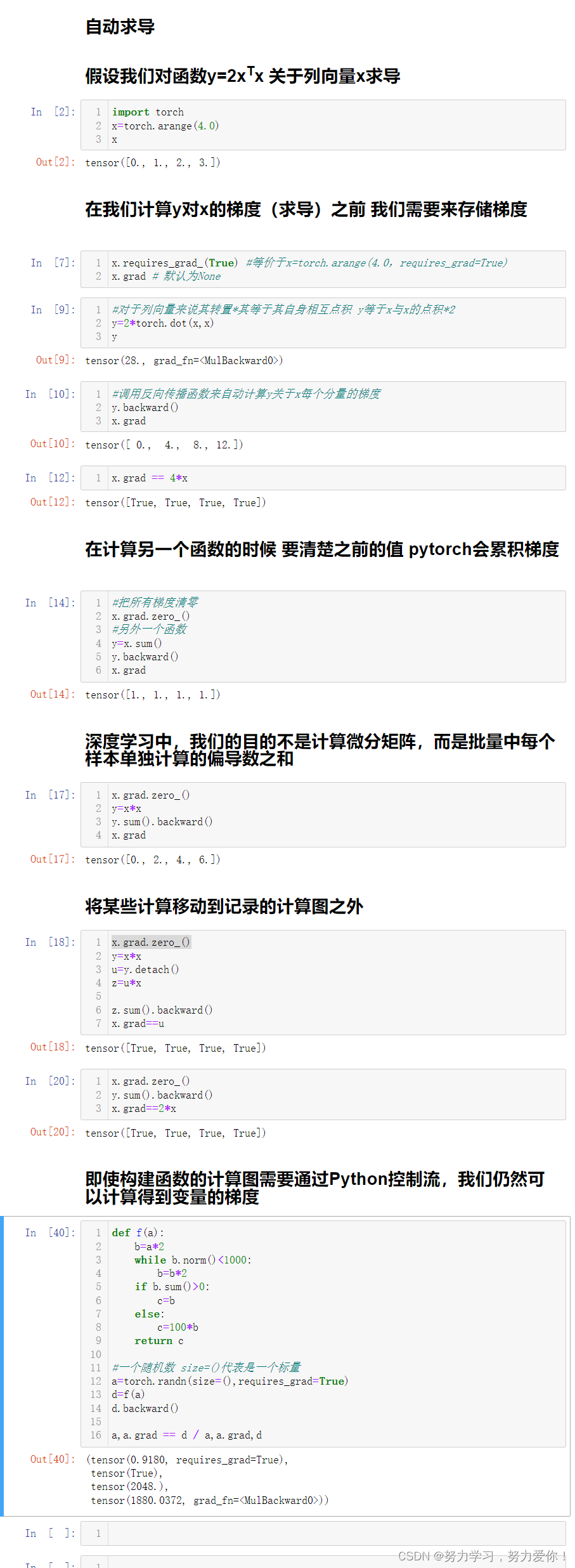
import torch
x=torch.arange(4.0)
x

在我们计算y对x的梯度（求导）之前 我们需要来存储梯度

x.requires_grad_(True) #等价于x=torch.arange(4.0，requires_grad=True)
x.grad # 默认为None
#对于列向量来说其转置*其等于其自身相互点积 y等于x与x的点积*2 
y=2*torch.dot(x,x)
y
#调用反向传播函数来自动计算y关于x每个分量的梯度
y.backward()
x.grad
x.grad == 4*x

在计算另一个函数的时候 要清楚之前的值 pytorch会累积梯度

#把所有梯度清零
x.grad.zero_()
#另外一个函数
y=x.sum()
y.backward()
x.grad

深度学习中，我们的目的不是计算微分矩阵，而是批量中每个样本单独计算的偏导数之和

x.grad.zero_()
y=x*x
y.sum().backward()
x.grad

将某些计算移动到记录的计算图之外

x.grad.zero_()
y=x*x
u=y.detach()
z=u*xz.sum().backward()
x.grad==ux.grad.zero_()
y.sum().backward()
x.grad==2*x

即使构建函数的计算图需要通过Python控制流，我们仍然可以计算得到变量的梯度

def f(a):b=a*2while b.norm()<1000:b=b*2if b.sum()>0:c=belse:c=100*breturn c#一个随机数 size=()代表一个标量
a=torch.randn(size=(),requires_grad=True)
d=f(a)
d.backward()
a.grad==d/a

作者声明

如有问题，欢迎指正！