Pytorch 复习总结,仅供笔者使用,参考教材:
- 《动手学深度学习》
- Stanford University: Practical Machine Learning
本文主要内容为:Pytorch 计算机视觉。
本文先介绍了计算机视觉中两种常见的改进模型泛化性能的方法:图像增广和模型微调,并将其应用于图像分类任务。然后介绍了几种计算机视觉的常见任务 —— 目标检测、风格迁移和语义分割。
Pytorch 语法汇总:
- Pytorch 张量的常见运算、线性代数、高等数学、概率论 部分 见 Pytorch 复习总结1;
- Pytorch 线性神经网络 部分 见 Pytorch 复习总结2;
- Pytorch 多层感知机 部分 见 Pytorch 复习总结3;
- Pytorch 深度学习计算 部分 见 Pytorch 复习总结4;
- Pytorch 卷积神经网络 部分 见 Pytorch 复习总结5;
- Pytorch 计算机视觉 部分 见 Pytorch 复习总结6;
目录
- 一. 图像增广
- 二. 模型微调
- 三. 目标检测
- 1. 边界框
- 2. 锚框
- 3. 交并比
- 四. 风格迁移
- 1. 图像读取和处理
- 2. 抽取图像特征
- 3. 损失函数
- 4. 初始化合成图像
- 5. 训练
- 五. 语义分割
- 1. Pascal VOC2012 数据集
- 2. 转置卷积
- 3. 全卷积网络
- 4. 损失函数
- 5. 训练
- 6. 预测
一. 图像增广
大型数据集是成功应用深度神经网络的先决条件,但并不是所有任务都有足够的训练数据。为了扩充训练数据集,让模型学习到更多的特征,从而提高模型鲁棒性、减少过拟合的风险,会对现有数据集做图像增广操作。
图像增广是指在不改变图像标签或含义的前提下,对图像进行一系列变换,以产生与原始图像相关但略有不同的图像。下面的示例代码展示了图像增广前后的变化,apply(img, aug, num_rows, num_cols, scale) 函数的 aug 参数可以替换成必要的增广方法:
import matplotlib.pyplot as plt
from PIL import Image
import torchvision.transforms as transformsimg = Image.open(r'data/img/cat1.jpg')
plt.imshow(img)
plt.show()def show_images(imgs, num_rows, num_cols, scale=1.5):figsize = (num_cols * scale, num_rows * scale)fig, axes = plt.subplots(num_rows, num_cols, figsize=figsize)for i in range(num_rows):for j in range(num_cols):axes[i][j].imshow(imgs[i * num_cols + j])axes[i][j].axes.get_xaxis().set_visible(False)  # 隐藏子图中X轴的刻度标签axes[i][j].axes.get_yaxis().set_visible(False)  # 隐藏子图中Y轴的刻度标签plt.show()def apply(img, aug, num_rows=2, num_cols=4, scale=1.5):Y = [aug(img) for _ in range(num_rows * num_cols)]      # 应用图像增广函数aug到原始图像img上show_images(Y, num_rows, num_cols, scale=scale)apply(img, transforms.RandomHorizontalFlip())
常见的图像增广技术包括但不限于:
- 随机旋转:在一定范围内随机旋转图像,使用
torchvision.transforms.RandomRotation(); - 随机缩放:对图像进行随机缩放,使其大小发生变化,使用
torchvision.transforms.RandomResizedCrop(size); - 随机平移:对图像进行随机平移,沿着水平和垂直方向移动图像,使用
torchvision.transforms.RandomAffine(degrees); - 镜像翻转:以一定概率对图像进行水平或垂直翻转,使用
torchvision.transforms.RandomHorizontalFlip()或torchvision.transforms.RandomVerticalFlip(); - 调整亮度和对比度:随机调整图像的亮度和对比度,使用
torchvision.transforms.ColorJitter(brightness, contrast, saturation, hue); - 裁剪:对图像进行随机裁剪或固定位置的裁剪,使用
torchvision.transforms.CenterCrop()、torchvision.transforms.RandomCrop()或torchvision.transforms.TenCrop();
除了上述介绍的方法,还可以通过添加噪声、变换颜色空间等方法增广图像。如果想要结合多种图像增广方法,可以使用 Compose 实例来综合不同的图像增广方法:
shape_aug = transforms.RandomResizedCrop((200, 200), scale=(0.1, 1), ratio=(0.5, 2))
color_aug = transforms.ColorJitter(brightness=0.5, contrast=0.5, saturation=0.5, hue=0.5)
flip_aug = transforms.RandomHorizontalFlip()
augs = transforms.Compose([flip_aug, color_aug, shape_aug])
apply(img, augs)
因为 卷积神经网络通常接受的输入数据格式是一个四维张量,通常形状为 (batch_size, channels, height, width),所以图像增广后一般会接 .unsqueeze(0) 操作将单张图像转换为批次维度为 1 的张量,从而能够传入卷积神经网络进行处理。
二. 模型微调
在传统的机器学习中,模型通常是使用任务特定的数据集从头开始训练的。然而,这种方法往往存在一些限制:数据稀缺、训练过程耗费大量的时间和计算资源、模型的泛化性能受限等。迁移学习可以解决传统机器学习的上述缺陷,即通过以前学到的知识和经验来解决新问题,而不是完全从零开始学习。
迁移学习的目标是将从一个相关任务中学到的知识应用到另一个任务中,相关性可以体现在数据集的相似性、特征的相关性或任务的相似性上。迁移学习可以通过多种技术和方法来实现,如特征提取、微调、领域自适应、模型蒸馏、元学习等,本节主要介绍微调技术。

模型微调包括以下四个步骤:
- 在源数据集上预训练源模型;
- 创建目标模型,复制源模型上的所有模型设计及其参数(输出层除外);
- 在目标模型中添加输出层,其输出数是目标数据集中的类别数,然后随机初始化该层的模型参数;
- 在目标数据集上训练目标模型,输出层将从头开始进行训练,而所有其他层的参数仅根据源模型的参数进行微调;
下面以 ResNet-18 作为源模型,在自定义数据集上进行微调,训练过程使用 Pytorch 复习总结 5 中封装的函数 train_net_gpu(net, train_iter, test_iter, loss, num_epochs, optimizer, device):
import os
import torch
import torchvision
from torch import nn'''裁切随机大小和长宽比的区域并缩放为224x224像素, 再标准化RGB通道'''
train_augs = torchvision.transforms.Compose([torchvision.transforms.RandomResizedCrop(224),torchvision.transforms.RandomHorizontalFlip(),torchvision.transforms.ToTensor(),torchvision.transforms.Normalize([0.485, 0.456, 0.406], [0.229, 0.224, 0.225])
])
test_augs = torchvision.transforms.Compose([torchvision.transforms.Resize([256, 256]),torchvision.transforms.CenterCrop(224),torchvision.transforms.ToTensor(),torchvision.transforms.Normalize([0.485, 0.456, 0.406], [0.229, 0.224, 0.225])
])'''加载自己的数据集, 并增广图像'''
data_dir = r'data\hotdog'
# train_imgs = torchvision.datasets.ImageFolder(os.path.join(data_dir, 'train'))
# test_imgs = torchvision.datasets.ImageFolder(os.path.join(data_dir, 'test'))
batch_size=128
train_iter = torch.utils.data.DataLoader(torchvision.datasets.ImageFolder(os.path.join(data_dir, 'train'), transform=train_augs), batch_size=batch_size, shuffle=True)
test_iter = torch.utils.data.DataLoader(torchvision.datasets.ImageFolder(os.path.join(data_dir, 'test'), transform=test_augs), batch_size=batch_size)'''使用在ImageNet数据集上预训练的ResNet-18作为源模型, 并将输出数量被设置为目标数据集中的类数'''
finetune_net = torchvision.models.resnet18(pretrained=True)
finetune_net.fc = nn.Linear(finetune_net.fc.in_features, 2)
nn.init.xavier_uniform_(finetune_net.fc.weight)loss = nn.CrossEntropyLoss(reduction="none")
learning_rate = 5e-5    # 学习率
param_group = True      # 输出层中的模型参数使用十倍的学习率if param_group:params_1x = [param for name, param in finetune_net.named_parameters() if name not in ["fc.weight", "fc.bias"]]optimizer = torch.optim.SGD([{'params': params_1x}, {'params': finetune_net.fc.parameters(), 'lr': learning_rate * 10}],lr=learning_rate, weight_decay=0.001)
else:optimizer = torch.optim.SGD(finetune_net.parameters(), lr=learning_rate, weight_decay=0.001)'''训练'''
def accuracy(y_hat, y):if len(y_hat.shape) > 1 and y_hat.shape[1] > 1:y_hat = y_hat.argmax(axis=1)cmp = y_hat.type(y.dtype) == yreturn float(cmp.type(y.dtype).sum())
def evaluate_accuracy_gpu(net, data_iter, device):if isinstance(net, nn.Module):net.eval()          			# 设置为评估模式test_acc_sum = 0.0      			# 正确预测的数量test_sample_num = 0     			# 总预测的数量with torch.no_grad():for X, y in data_iter:if isinstance(X, list):X = [x.to(device) for x in X]else:X = X.to(device)y = y.to(device)test_acc_sum += accuracy(net(X), y)test_sample_num += y.numel()return test_acc_sum / test_sample_num
def train_net_gpu(net, train_iter, test_iter, loss, num_epochs, optimizer, device):net.to(device)for epoch in range(num_epochs):train_loss_sum = 0.0            # 训练损失总和train_acc_sum = 0.0             # 训练准确度总和sample_num = 0                  # 样本数net.train()for i, (X, y) in enumerate(train_iter):optimizer.zero_grad()X, y = X.to(device), y.to(device)y_hat = net(X)l = loss(y_hat, y)l.sum().backward()optimizer.step()with torch.no_grad():train_loss_sum += l.sum()train_acc_sum += accuracy(y_hat, y)sample_num += y.numel()train_loss = train_loss_sum / sample_numtrain_acc = train_acc_sum / sample_numtest_acc = evaluate_accuracy_gpu(net, test_iter, device)print(f'loss {train_loss:.3f}, train acc {train_acc:.3f}, test acc {test_acc:.3f}')device = torch.device('cuda:0' if torch.cuda.is_available() else 'cpu')
print('---------------- training on', device, '----------------')
num_epochs = 5
train_net_gpu(finetune_net, train_iter, test_iter, loss, num_epochs, optimizer, device)
'''
---------------- training on cuda:0 ----------------
loss 2.741, train acc 0.676, test acc 0.926
loss 0.329, train acc 0.910, test acc 0.818
loss 0.270, train acc 0.910, test acc 0.932
loss 0.230, train acc 0.919, test acc 0.926
loss 0.226, train acc 0.918, test acc 0.941
'''
三. 目标检测
目标检测 (object detection) 是计算机视觉领域的一个重要任务,旨在识别图像中的特定物体并确定其在图像中的位置和边界框。其主要目标是检测图像中的多个目标,并标记出它们的位置和类别。
1. 边界框
在目标检测任务中,通常使用边界框 (bounding box) 来描述对象的空间位置。边界框是矩形的,有两种表示方法:一种是由矩形左上角到以及右下角的 ( x , y ) (x, y) (x,y) 坐标决定;另一种是边界框中心坐标以及框的宽度和高度。这两种方法可以互相转换:
def box_corner_to_center(boxes):"""从(左上,右下)转换到(中间,宽度,高度)"""x1, y1, x2, y2 = boxes[:, 0], boxes[:, 1], boxes[:, 2], boxes[:, 3]cx = (x1 + x2) / 2cy = (y1 + y2) / 2w = x2 - x1h = y2 - y1boxes = torch.stack((cx, cy, w, h), axis=-1)return boxesdef box_center_to_corner(boxes):"""从(中间,宽度,高度)转换到(左上,右下)"""cx, cy, w, h = boxes[:, 0], boxes[:, 1], boxes[:, 2], boxes[:, 3]x1 = cx - 0.5 * wy1 = cy - 0.5 * hx2 = cx + 0.5 * wy2 = cy + 0.5 * hboxes = torch.stack((x1, y1, x2, y2), axis=-1)return boxesboxes = torch.tensor([[1,1,3,5], [4,2,6,6]])	# 批量操作
print(box_corner_to_center(boxes))
需要注意的是,目标检测一般使用 屏幕坐标系统,坐标系是以 左上角为原点,x 轴向右为正,y 轴向下为正的坐标系。所以
box_corner_to_center(boxes)中的h = y2 - y1而不是h = y1 - y2。
下面示例代码使用 matplotlib 将边界框在图像中画出,因为 matplotlib 的边界框还是采用的平面直角坐标系格式,所以还需要一定的格式转换:
import matplotlib.pyplot as plt
from PIL import Imageimg = Image.open(r'data/img/catdog.jpg')
fig = plt.imshow(img)def bbox_to_rect(bbox, color):# 将边界框(左上x, 左上y, 右下x, 右下y)转换成matplotlib格式((左上x,左上y),宽,高)return plt.Rectangle(xy=(bbox[0], bbox[1]), width=bbox[2]-bbox[0], height=bbox[3]-bbox[1],fill=False, edgecolor=color, linewidth=2)dog_bbox, cat_bbox = [60.0, 45.0, 378.0, 516.0], [400.0, 112.0, 655.0, 493.0]fig.axes.add_patch(bbox_to_rect(dog_bbox, 'blue'))
fig.axes.add_patch(bbox_to_rect(cat_bbox, 'red'))
plt.show()

2. 锚框
在目标检测任务中,如果想要在图像中定位和分类物体,需要先生成一些候选区域 (Region of Interest, ROI) 再进行检测,这些候选区域称为锚框 (Anchor Box) 或先验框 (Prior Box)。通过在不同位置、尺度和宽高比的图像区域生成多个锚框,这些锚框可能覆盖多个可能存在物体的区域,然后算法根据这些锚框进行目标检测。
不同的模型使用的区域采样方法可能不同,这里介绍其中的一种方法:以每个像素为中心,生成多个缩放比 (scale) 和宽高比 (aspect ratio) 不同的锚框。设图像高度为 h h h,宽度为 w w w,缩放比取值为 s 1 , s 2 , ⋯ , s n s_1, s_2, \cdots, s_n s1,s2,⋯,sn,宽高比取值为 r 1 , r 2 , ⋯ , r m r_1, r_2, \cdots, r_m r1,r2,⋯,rm,则以每个像素为中心可以生成 n m nm nm 个锚框,整张图像可以生成 w h n m whnm whnm 个锚框。这些锚框显然覆盖了所有目标可能出现的区域,但由于计算复杂度太高,实际应用中一般只考虑包含 s 1 s_1 s1 或 r 1 r_1 r1 的组合,以每个像素为中心生成 n + m − 1 n+m-1 n+m−1 个锚框。锚框宽度和高度分别为 h s r hs\sqrt r hsr 和 h s / r hs / \sqrt r hs/r。
生成以每个像素为中心具有不同形状的锚框过程如下:
import torch
import matplotlib.pyplot as plt"""生成以每个像素为中心具有不同形状的锚框"""
def multibox_prior(data, scales, ratios):# 读取输入变量in_height, in_width = data.shape[-2:]device, num_scales, num_ratios = data.device, len(scales), len(ratios)boxes_per_pixel = num_scales + num_ratios - 1size_tensor = torch.tensor(scales, device=device)ratio_tensor = torch.tensor(ratios, device=device)# 设置偏移量以将锚点移动到像素中心offset_h, offset_w = 0.5, 0.5steps_h = 1.0 / in_height   # 在y轴上缩放步长steps_w = 1.0 / in_width    # 在x轴上缩放步长# 生成锚框的所有中心点center_h = (torch.arange(in_height, device=device) + offset_h) * steps_hcenter_w = (torch.arange(in_width, device=device) + offset_w) * steps_wshift_y, shift_x = torch.meshgrid(center_h, center_w, indexing='ij')    # 生成两个张量的网格shift_y, shift_x = shift_y.reshape(-1), shift_x.reshape(-1)             # 展开# 生成含所有锚框中心的网格,重复boxes_per_pixel次out_grid = torch.stack([shift_x, shift_y, shift_x, shift_y],dim=1).repeat_interleave(boxes_per_pixel, dim=0)# 生成boxes_per_pixel个高和宽w = torch.cat((size_tensor * torch.sqrt(ratio_tensor[0]), size_tensor[0] * torch.sqrt(ratio_tensor[1:])))h = torch.cat((size_tensor / torch.sqrt(ratio_tensor[0]), size_tensor[0] / torch.sqrt(ratio_tensor[1:])))w *= in_height / in_width   # 处理矩形输入print(w, h)                 # tensor([0.5780, 0.3853, 0.1927, 0.8173, 0.4087]) tensor([0.7500, 0.5000, 0.2500, 0.5303, 1.0607])# 创建锚框相对中心点的四角坐标anchor_manipulations = torch.stack((-w, -h, w, h)).T.repeat(in_height * in_width, 1) / 2# 计算锚框的四角坐标output = out_grid + anchor_manipulationsreturn output.unsqueeze(0)  # 在张量的最外层添加一个维度img = plt.imread(r'data/img/catdog.jpg')
height, width, channels = img.shape                 # 561 728 3
batch_size = 1                                      # 图像数量
X = torch.rand(size=(batch_size, channels, height, width))
scales=[0.75, 0.5, 0.25]                            # 缩放比
ratios=[1, 2, 0.5]                                  # 宽高比
boxes_per_pixel = len(scales) + len(ratios) - 1     # 以每个像素为中心的锚框个数Y = multibox_prior(X, scales, ratios)
print(Y.shape)                  # torch.Size([1, 2042040, 4])
boxes = Y.reshape(height, width, boxes_per_pixel, 4)
print(boxes[0][0][0])           # tensor([-0.2883, -0.3741,  0.2897,  0.3759])
以像素点 (250, 250) 为例,在图像上绘制所有锚框:
def show_bboxes(axes, bboxes, labels=None, colors=None):def _make_list(obj, default_values=None):if obj is None:obj = default_valueselif not isinstance(obj, (list, tuple)):obj = [obj]return objdef bbox_to_rect(bbox, color):return plt.Rectangle(xy=(bbox[0], bbox[1]), width=bbox[2]-bbox[0], height=bbox[3]-bbox[1],fill=False, edgecolor=color, linewidth=2)labels = _make_list(labels)colors = _make_list(colors, ['b', 'g', 'r', 'm', 'c'])for i, bbox in enumerate(bboxes):color = colors[i % len(colors)]rect = bbox_to_rect(bbox.detach().numpy(), color)axes.add_patch(rect)if labels and len(labels) > i:text_color = 'k' if color == 'w' else 'w'axes.text(rect.xy[0], rect.xy[1], labels[i],va='center', ha='center', fontsize=9, color=text_color,bbox=dict(facecolor=color, lw=0))plt.figure(figsize=(8, 6))
bbox_scale = torch.tensor((width, height, width, height))
fig = plt.imshow(img)
show_bboxes(fig.axes, boxes[250, 250, :, :] * bbox_scale,['s=0.75, r=1', 's=0.5, r=1', 's=0.25, r=1', 's=0.75, r=2', 's=0.75, r=0.5'])
plt.show()

3. 交并比
在训练集中,每个锚框都会被视为一个训练样本,结合每个锚框的类别和偏移量标签,训练模型输出符合特定条件的预测边界框。为了衡量锚框与真实边界框之间的相似性,引入了杰卡德系数 (Jaccard),也称为交并比 (intersection over union, IoU)。两个边界框的相似性等于它们交集的大小除以并集的大小:

import torchdef box_iou(boxes1, boxes2):"""计算两个锚框或边界框列表中成对的交并比"""box_area = lambda boxes: ((boxes[:, 2] - boxes[:, 0]) * (boxes[:, 3] - boxes[:, 1]))# boxes1,boxes2,areas1,areas2的形状:# boxes1:(boxes1的数量,4),# boxes2:(boxes2的数量,4),# areas1:(boxes1的数量,),# areas2:(boxes2的数量,)areas1 = box_area(boxes1)areas2 = box_area(boxes2)# inter_upperlefts,inter_lowerrights,inters的形状:# (boxes1的数量,boxes2的数量,2)inter_upperlefts = torch.max(boxes1[:, None, :2], boxes2[:, :2])inter_lowerrights = torch.min(boxes1[:, None, 2:], boxes2[:, 2:])inters = (inter_lowerrights - inter_upperlefts).clamp(min=0)# inter_areasandunion_areas的形状:(boxes1的数量,boxes2的数量)inter_areas = inters[:, :, 0] * inters[:, :, 1]union_areas = areas1[:, None] + areas2 - inter_areasreturn inter_areas / union_areasboxes1, boxes2 = torch.tensor([[1,1,2,5],[2,2,4,4]]), torch.tensor([[1,2,4,5],[3,3,6,6]])
print(box_iou(boxes1, boxes2))
'''
tensor([[0.3000, 0.0000],[0.4444, 0.0833]])
'''
更多目标检测算法见 13.4. 锚框 ~ 13.8. 区域卷积神经网络(R-CNN)系列 。
四. 风格迁移
风格迁移 (style transfer) 是一种图像处理技术,旨在将一张图像的风格转移到另一张图像上,从而创造出具有原始图像内容和目标图像风格的新图像。风格迁移的基本思想是将图像分解为内容和风格两个部分,然后通过优化目标函数,使得合成图像在内容上接近于原始图像,而在风格上接近于目标图像。

风格迁移一般将合成图像初始化为内容图像,使用预训练的卷积神经网络凭借多个层逐级抽取抽取样式图像的风格,然后将其应用于合成图像。整个过程中只有合成图像需要迭代更新,卷积神经网络的参数保持不变。
1. 图像读取和处理
读取图像:
from PIL import Image'''读取图像'''
content_img = Image.open(r'data\img\rainier.jpg')
style_img = Image.open(r'data\img\autumn-oak.jpg')
读取图像后,需要对图像进行预处理:对输入图像在 RGB 三个通道分别做标准化,并将结果变换成卷积神经网络接受的输入格式。图像预处理的过程只是为了让卷积神经网络比较好处理,没有实际的物理意义:
import torch
import torchvision'''图像预处理'''
rgb_mean = torch.tensor([0.485, 0.456, 0.406])
rgb_std = torch.tensor([0.229, 0.224, 0.225])
def preprocess(img, image_shape):transforms = torchvision.transforms.Compose([torchvision.transforms.Resize(image_shape),torchvision.transforms.ToTensor(),torchvision.transforms.Normalize(mean=rgb_mean, std=rgb_std)])return transforms(img).unsqueeze(0)     # 将单张图像转换为批次维度为1的张量
合成图像经过卷积神经网络处理后,需要进行图像后处理:将张量格式的图像再转换回 PIL 图像格式,并进行一些标准化操作的逆过程。由于图像打印函数要求每个像素的浮点数值在 0~1 之间,因此对小于 0 和大于 1 的值分别取 0 和 1:
'''图像后处理'''
def postprocess(img):img = img[0].to(rgb_std.device)img = img.permute(1, 2, 0) * rgb_std + rgb_mean     # 反标准化img = torch.clamp(img, 0, 1)            # 将张量中的值限制在[0, 1]内return torchvision.transforms.ToPILImage()(img.permute(2, 0, 1))
2. 抽取图像特征
本节使用基于 ImageNet 数据集预训练的 VGG-19 模型来抽取图像特征。在图像风格迁移的过程中,选择网络中不同层的输出可以得到不同层次的特征表示:选择网络中较靠近 输入层 的层输出可以抽取更多的图像细节信息,如图像的 纹理、颜色 等细节特征;而选择网络中较靠近 输出层 的层输出则更容易抽取图像的全局信息,如图像的 全局信息和结构。VGG 网络 使用了 5 个卷积块,本节选择第 4 卷积块的最后一个卷积层作为内容层,选择每个卷积块的第一个卷积层作为风格层:
'''抽取图像特征'''
pretrained_net = torchvision.models.vgg19(pretrained=True)
style_layers, content_layers = [0, 5, 10, 19, 28], [25]
net = nn.Sequential(*[pretrained_net.features[i] for i in range(max(content_layers + style_layers) + 1)]
)
为了得到中间层的输出,需要逐层计算,并保留内容层和风格层的所有输出:
def extract_features(X, content_layers, style_layers):contents = []styles = []for i in range(len(net)):X = net[i](X)if i in style_layers:styles.append(X)if i in content_layers:contents.append(X)return contents, styles
因为训练时无须改变预训练的 VGG 模型参数,所以在训练开始之前就可以提取出内容图像和风格图像的内容特征和风格特征:
def get_contents(image_shape, device):content_X = preprocess(content_img, image_shape).to(device)contents_Y, _ = extract_features(content_X, content_layers, style_layers)return content_X, contents_Ydef get_styles(image_shape, device):style_X = preprocess(style_img, image_shape).to(device)_, styles_Y = extract_features(style_X, content_layers, style_layers)return style_X, styles_Y
3. 损失函数
风格迁移任务的损失函数由三部分组成:
- 内容损失:使用
extract_features函数计算得到合成图像和内容图像的内容特征的平方误差。通过优化内容损失使合成图像与内容图像在内容特征上接近; - 风格损失:使用
extract_features函数计算得到合成图像和风格图像的风格特征的平方误差,风格层的输出风格由格拉姆矩阵表示。通过优化风格损失使合成图像与风格图像在风格特征上接近; - 全变分损失:有助于减少合成图像中的高频噪点(特别亮或者特别暗的颗粒像素);
'''损失函数'''
def content_loss(Y_hat, Y):return torch.square(Y_hat - Y.detach()).mean()  # 从动态计算梯度的树中分离Y
def gram(X):num_channels, n = X.shape[1], X.numel() // X.shape[1]X = X.reshape((num_channels, n))return torch.matmul(X, X.T) / (num_channels * n)
def style_loss(Y_hat, gram_Y):return torch.square(gram(Y_hat) - gram_Y.detach()).mean()
def tv_loss(Y_hat):return 0.5 * (torch.abs(Y_hat[:, :, 1:, :] - Y_hat[:, :, :-1, :]).mean() +torch.abs(Y_hat[:, :, :, 1:] - Y_hat[:, :, :, :-1]).mean())content_weight, style_weight, tv_weight = 1, 1e3, 10
def compute_loss(X, contents_Y_hat, styles_Y_hat, contents_Y, styles_Y_gram):contents_l = [content_loss(Y_hat, Y) * content_weight for Y_hat, Y in zip(contents_Y_hat, contents_Y)]styles_l = [style_loss(Y_hat, Y) * style_weight for Y_hat, Y in zip(styles_Y_hat, styles_Y_gram)]tv_l = tv_loss(X) * tv_weightl = sum(10 * styles_l + contents_l + [tv_l])    # 对所有损失求和return contents_l, styles_l, tv_l, l
4. 初始化合成图像
在风格迁移任务中,预训练网络不需要更新参数,合成图像是训练期间唯一需要更新的变量。为了让能够更新合成图像,将其封装为 SynthesizedImage 类。nn.Parameter 用于将张量包装成模型的参数,使得在模型优化过程中可以自动更新:
'''初始化合成图像'''
class SynthesizedImage(nn.Module):def __init__(self, img_shape, **kwargs):super(SynthesizedImage, self).__init__(**kwargs)self.weight = nn.Parameter(torch.rand(*img_shape))def forward(self):return self.weight
随后初始化合成图像为内容图像,并定义优化器指定反向传播时要更新的参数:
def get_inits(X, device, lr, styles_Y):gen_img = SynthesizedImage(X.shape).to(device)gen_img.weight.data.copy_(X.data)optimizer = torch.optim.Adam(gen_img.parameters(), lr=lr)styles_Y_gram = [gram(Y) for Y in styles_Y]return gen_img(), styles_Y_gram, optimizer
5. 训练
训练模型进行风格迁移时,循环抽取合成图像的内容特征和风格特征并计算损失:
'''训练模型'''
def train(X, contents_Y, styles_Y, device, lr, num_epochs, lr_decay_epoch):X, styles_Y_gram, trainer = get_inits(X, device, lr, styles_Y)scheduler = torch.optim.lr_scheduler.StepLR(trainer, lr_decay_epoch, 0.8)for epoch in range(num_epochs):trainer.zero_grad()contents_Y_hat, styles_Y_hat = extract_features(X, content_layers, style_layers)contents_l, styles_l, tv_l, l = compute_loss(X, contents_Y_hat, styles_Y_hat, contents_Y, styles_Y_gram)l.sum().backward()trainer.step()scheduler.step()if (epoch + 1) % 50 == 0:print(f'epoch {epoch+1}: loss {l:.3f}')return Xdevice = torch.device('cuda:0' if torch.cuda.is_available() else 'cpu')
image_shape = (300, 450)
net = net.to(device)
content_X, contents_Y = get_contents(image_shape, device)
styles_X, styles_Y = get_styles(image_shape, device)
output = train(content_X, contents_Y, styles_Y, device, 0.3, 1000, 50)
'''
epoch 50: loss 6.738
epoch 100: loss 4.740
epoch 150: loss 3.419
epoch 200: loss 3.045
epoch 250: loss 2.763
epoch 300: loss 2.674
epoch 350: loss 2.580
epoch 400: loss 2.410
epoch 450: loss 2.367
epoch 500: loss 2.334
epoch 550: loss 2.316
epoch 600: loss 2.299
epoch 650: loss 2.286
epoch 700: loss 2.277
epoch 750: loss 2.269
epoch 800: loss 2.263
epoch 850: loss 2.258
epoch 900: loss 2.254
epoch 950: loss 2.251
epoch 1000: loss 2.248
'''
print(type(output))         # <class 'torch.nn.parameter.Parameter'>
网络的输出结果 output 是参数对象,对其后处理后才能够可视化:
'''可视化合成图像'''
import matplotlib.pyplot as plt
plt.imshow(postprocess(output))
plt.show()

五. 语义分割
语义分割 (semantic segmentation) 是计算机视觉中的一项重要任务,旨在将图像中的每个像素分配到其对应的语义类别中,以区分不同的语义区域。与目标检测不同,语义分割不仅要识别图像中的物体,还需要对每个像素进行分类,从而实现对图像的像素级别理解。

图像分割 & 语义分割 & 实例分割:
- 图像分割:利用图像中像素之间的相关性将图像划分为若干个区域,而不需要考虑像素的标签信息。以上图为例,图像分割可能会将狗分为两个区域:一个覆盖以黑色为主的嘴和眼睛,另一个覆盖以黄色为主的其余部分身体。
- 语义分割:图像分割的一种特殊形式,不仅仅将图像分割成区域,还为图像中的每个像素分配一个类别标签,以表示该像素属于图像中的哪个语义类别。语义分割提供了对图像像素的语义理解,但不区分不同实例(即相同类别的不同个体)。以上图为例,语义分割会将图像分为三个区域:猫、狗和背景。
- 实例分割:语义分割的一种特殊形式,不仅提供了图像中对象的像素级别分割,还在图像中识别和分割出各个对象的特定实例。即使是同一类别,实例分割也能够区分不同对象之间的边界,并为每个对象分配唯一的标识符。如果图像中有两条狗,那么实例分割可以区分像素属于的两条狗中的哪一条。
1. Pascal VOC2012 数据集
Pascal VOC2012 数据集 是一个经典的计算机视觉数据集,用于目标检测、语义分割和图像分类等任务的训练和评估。该数据集包含了 20 个常见的物体类别,包括人、动物、车辆、家具等,每个图像都有一个或多个对象的标注,以及这些对象的边界框和类别标签。此外,Pascal VOC2012 数据集还提供了每张图像的语义分割标注,数据集结构如下:
├─VOCdevkit
|   ├─VOC2012
|   |   ├─Annotations:包含目标检测和物体识别任务的标注数据,以 XML 格式存储,每个 XML 文件包含边界框的位置、对象类别等信息;
|   |   ├─ImageSets:包含用于不同任务的训练(train.txt)、验证(val.txt)及其组合(trainval.txt)的图像集合的列表;
|   |   |   ├─Action:用于动作识别任务的图像集合列表;
|   |   |   ├─Layout:用于布局分析任务的图像集合列表;
|   |   |   ├─Main:用于目标检测、物体识别等主要任务的图像集合列表;
|   |   |   └ Segmentation:用于语义分割和实例分割任务的图像集合列表;
|   |   ├─JPEGImages:包含原始的JPEG格式图像文件;
|   |   ├─SegmentationClass:包含语义分割的标注信息,用于每个像素的类别标签;
|   |   └ SegmentationObject:包含实例分割的标注信息,用于每个像素的对象标识符;
读取 VOC2012 数据集代码如下:
import os
import torch
import torchvisiondef read_voc_images(voc_dir, is_train=True):"""读取所有VOC图像并标注"""txt_fname = os.path.join(voc_dir, 'ImageSets', 'Segmentation','train.txt' if is_train else 'val.txt')mode = torchvision.io.image.ImageReadMode.RGB       # 指定图像以RGB格式读取with open(txt_fname, 'r') as f:images = f.read().split()features, labels = [], []for i, fname in enumerate(images):features.append(torchvision.io.read_image(os.path.join(voc_dir, 'JPEGImages', f'{fname}.jpg')))labels.append(torchvision.io.read_image(os.path.join(voc_dir, 'SegmentationClass' ,f'{fname}.png'), mode))return features, labels'''读取数据集'''
voc_dir = r'data\VOCdevkit\VOC2012'
train_features, train_labels = read_voc_images(voc_dir, True)
print(train_features[0].shape,train_labels[0].shape)    # torch.Size([3, 281, 500]) torch.Size([3, 281, 500])'''可视化'''
import torchvision.transforms as transforms
import matplotlib.pyplot as plt
img = train_features[0] + train_labels[0]				# 将标签
img = img.permute(1,2,0)            # 重排原始张量的维度,第一维度变为第二维度,第二维度变为第三维度,第三维度变为第一维度
plt.imshow(img.numpy())
plt.axis('off')
plt.show()
此处的 标签也采用图像格式,尺寸与原始图像相同,标签中颜色相同的像素属于同一个语义类别。将标签加到原始图像上可视化如下:

为了构建标签的 RGB 颜色值到类别索引的映射,以及 RGB 颜色值到数据集中类别索引的映射,定义函数如下:
'''构建VOC标签中的RGB值到类别索引的映射'''
VOC_COLORMAP = [[0, 0, 0], [128, 0, 0], [0, 128, 0], [128, 128, 0],[0, 0, 128], [128, 0, 128], [0, 128, 128], [128, 128, 128],[64, 0, 0], [192, 0, 0], [64, 128, 0], [192, 128, 0],[64, 0, 128], [192, 0, 128], [64, 128, 128], [192, 128, 128],[0, 64, 0], [128, 64, 0], [0, 192, 0], [128, 192, 0],[0, 64, 128]]
VOC_CLASSES = ['background', 'aeroplane', 'bicycle', 'bird', 'boat', 'bottle', 'bus', 'car','cat', 'chair', 'cow', 'diningtable','dog', 'horse', 'motorbike', 'person','potted plant', 'sheep', 'sofa', 'train','tv/monitor']
def voc_colormap2label():"""构建从RGB到VOC类别索引的映射"""colormap2label = torch.zeros(256 ** 3, dtype=torch.long)for i, colormap in enumerate(VOC_COLORMAP):colormap2label[(colormap[0] * 256 + colormap[1]) * 256 + colormap[2]] = ireturn colormap2label
def voc_label_indices(colormap, colormap2label):"""将VOC标签中的RGB值映射到它们的类别索引"""colormap = colormap.permute(1, 2, 0).numpy().astype('int32')idx = ((colormap[:, :, 0] * 256 + colormap[:, :, 1]) * 256 + colormap[:, :, 2])return colormap2label[idx]colormap2label = voc_colormap2label()
y = voc_label_indices(train_labels[0], colormap2label)
print(VOC_CLASSES[y[0][0]])         # background
将上述读取过程封装成类和函数,并对图像进行增广。以后使用时直接调用 load_data_voc(batch_size, crop_size) 函数就可以得到训练集和测试集的数据迭代器:
import os
import torch
import torchvisiondef read_voc_images(voc_dir, is_train=True):"""读取所有VOC图像并标注"""txt_fname = os.path.join(voc_dir, 'ImageSets', 'Segmentation','train.txt' if is_train else 'val.txt')mode = torchvision.io.image.ImageReadMode.RGB       # 指定图像以RGB格式读取with open(txt_fname, 'r') as f:images = f.read().split()features, labels = [], []for i, fname in enumerate(images):features.append(torchvision.io.read_image(os.path.join(voc_dir, 'JPEGImages', f'{fname}.jpg')))labels.append(torchvision.io.read_image(os.path.join(voc_dir, 'SegmentationClass' ,f'{fname}.png'), mode))return features, labels'''构建VOC标签中的RGB值到类别索引的映射'''
VOC_COLORMAP = [[0, 0, 0], [128, 0, 0], [0, 128, 0], [128, 128, 0],[0, 0, 128], [128, 0, 128], [0, 128, 128], [128, 128, 128],[64, 0, 0], [192, 0, 0], [64, 128, 0], [192, 128, 0],[64, 0, 128], [192, 0, 128], [64, 128, 128], [192, 128, 128],[0, 64, 0], [128, 64, 0], [0, 192, 0], [128, 192, 0],[0, 64, 128]]
VOC_CLASSES = ['background', 'aeroplane', 'bicycle', 'bird', 'boat', 'bottle', 'bus', 'car','cat', 'chair', 'cow', 'diningtable','dog', 'horse', 'motorbike', 'person','potted plant', 'sheep', 'sofa', 'train','tv/monitor']
def voc_colormap2label():"""构建从RGB到VOC类别索引的映射"""colormap2label = torch.zeros(256 ** 3, dtype=torch.long)for i, colormap in enumerate(VOC_COLORMAP):colormap2label[(colormap[0] * 256 + colormap[1]) * 256 + colormap[2]] = ireturn colormap2label
def voc_label_indices(colormap, colormap2label):"""将VOC标签中的RGB值映射到它们的类别索引"""colormap = colormap.permute(1, 2, 0).numpy().astype('int32')idx = ((colormap[:, :, 0] * 256 + colormap[:, :, 1]) * 256 + colormap[:, :, 2])return colormap2label[idx]def voc_rand_crop(feature, label, height, width):"""随机裁剪特征和标签图像"""rect = torchvision.transforms.RandomCrop.get_params(feature, (height, width))feature = torchvision.transforms.functional.crop(feature, *rect)label = torchvision.transforms.functional.crop(label, *rect)return feature, labelclass VOCSegDataset(torch.utils.data.Dataset):"""一个用于加载VOC数据集的自定义数据集"""def __init__(self, is_train, crop_size, voc_dir):self.transform = torchvision.transforms.Normalize(mean=[0.485, 0.456, 0.406], std=[0.229, 0.224, 0.225])self.crop_size = crop_sizefeatures, labels = read_voc_images(voc_dir, is_train=is_train)self.features = [self.normalize_image(feature)for feature in self.filter(features)]self.labels = self.filter(labels)self.colormap2label = voc_colormap2label()# print('read ' + str(len(self.features)) + ' examples')def normalize_image(self, img):return self.transform(img.float() / 255)def filter(self, imgs):return [img for img in imgs if (img.shape[1] >= self.crop_size[0] andimg.shape[2] >= self.crop_size[1])]def __getitem__(self, idx):feature, label = voc_rand_crop(self.features[idx], self.labels[idx],*self.crop_size)return (feature, voc_label_indices(label, self.colormap2label))def __len__(self):return len(self.features)def load_data_voc(batch_size, crop_size):"""加载VOC语义分割数据集"""voc_dir = r'data\VOCdevkit\VOC2012'num_workers = 4train_iter = torch.utils.data.DataLoader(VOCSegDataset(True, crop_size, voc_dir), batch_size,shuffle=True, drop_last=True, num_workers=num_workers)test_iter = torch.utils.data.DataLoader(VOCSegDataset(False, crop_size, voc_dir), batch_size,drop_last=True, num_workers=num_workers)return train_iter, test_iterbatch_size = 32
crop_size = (320, 480)
train_iter, test_iter = load_data_voc(batch_size, crop_size)
2. 转置卷积
计算机视觉任务中常常引入卷积层和池化层对图像进行下采样,从而提取图像特征。然而,像素级分类的语义分割任务显然需要输出原始尺寸的图像,这样才能为每个像素标注语义类别。因此,引入了 转置卷积 (transposed convolution),用于逆转下采样导致的空间尺寸减小。

转置卷积层可以通过 nn.ConvTranspose2d 实例化,示例如下:
import torch
from torch import nnX = torch.tensor([[[[0.0, 1.0], [2.0, 3.0]]]])
K = torch.tensor([[[[0.0, 1.0], [2.0, 3.0]]]])
tconv = nn.ConvTranspose2d(1, 1, kernel_size=2, bias=False)
tconv.weight.data = K
print(tconv(X))
'''
tensor([[[[ 0.,  0.,  1.],[ 0.,  4.,  6.],[ 4., 12.,  9.]]]], grad_fn=<ConvolutionBackward0>)
'''
3. 全卷积网络
全卷积网络 (fully convolutional network, FCN) 采用卷积神经网络可以实现从图像像素到像素类别的变换。与此前图像分类或目标检测任务中的卷积神经网络不同,全卷积网络通过转置卷积层将中间层特征图的高和宽变换回输入图像的尺寸。此外,为了将特征图的通道数调整到与语义类别数相匹配,在卷积神经网络的最后一层后一般会再添加一个 1x1 卷积层,输出特征图的每个通道对应一个语义类别的概率。

此处直接使用在 ImageNet 数据集上预训练的 ResNet-18 模型来提取图像特征,除了最后几层全局平均池化层和全连接层。然后添加 1×1 卷积层将输出通道数转换为 Pascal VOC2012 数据集的类数,再添加转置卷积层将特征图的高度和宽度变回输入图像的高和宽。转置卷积层的上采样采用双线性插值,内核由 bilinear_kernel 函数实现:
pretrained_net = torchvision.models.resnet18(pretrained=True)
net = nn.Sequential(*list(pretrained_net.children())[:-2])
num_classes = 21
net.add_module('final_conv', nn.Conv2d(512, num_classes, kernel_size=1))
net.add_module('transpose_conv', nn.ConvTranspose2d(num_classes, num_classes,kernel_size=64, padding=16, stride=32))def bilinear_kernel(in_channels, out_channels, kernel_size):factor = (kernel_size + 1) // 2if kernel_size % 2 == 1:center = factor - 1else:center = factor - 0.5og = (torch.arange(kernel_size).reshape(-1, 1), torch.arange(kernel_size).reshape(1, -1))filt = (1 - torch.abs(og[0] - center) / factor) * (1 - torch.abs(og[1] - center) / factor)weight = torch.zeros((in_channels, out_channels, kernel_size, kernel_size))weight[range(in_channels), range(out_channels), :, :] = filtreturn weight
W = bilinear_kernel(num_classes, num_classes, 64)
net.transpose_conv.weight.data.copy_(W)
4. 损失函数
因为模型中增加了输出特征图的通道来预测像素的语义类别,所以需要在损失计算中指定通道维。此外,模型基于每个像素的预测类别是否正确来计算准确率:
def loss(inputs, targets):return F.cross_entropy(inputs, targets, reduction='none').mean(1).mean(1)
5. 训练
训练过程使用 Pytorch 复习总结 5 中封装的函数 train_net_gpu(net, train_iter, test_iter, loss, num_epochs, optimizer, device),将训练好的模型参数写入 .pth 文件:
import os
import torch
import torchvision
from torch import nn
from torch.nn import functional as F'''加载VOC数据集'''
def read_voc_images(voc_dir, is_train=True):txt_fname = os.path.join(voc_dir, 'ImageSets', 'Segmentation','train.txt' if is_train else 'val.txt')mode = torchvision.io.image.ImageReadMode.RGB       # 指定图像以RGB格式读取with open(txt_fname, 'r') as f:images = f.read().split()features, labels = [], []for i, fname in enumerate(images):features.append(torchvision.io.read_image(os.path.join(voc_dir, 'JPEGImages', f'{fname}.jpg')))labels.append(torchvision.io.read_image(os.path.join(voc_dir, 'SegmentationClass' ,f'{fname}.png'), mode))return features, labels
VOC_COLORMAP = [[0, 0, 0], [128, 0, 0], [0, 128, 0], [128, 128, 0],[0, 0, 128], [128, 0, 128], [0, 128, 128], [128, 128, 128],[64, 0, 0], [192, 0, 0], [64, 128, 0], [192, 128, 0],[64, 0, 128], [192, 0, 128], [64, 128, 128], [192, 128, 128],[0, 64, 0], [128, 64, 0], [0, 192, 0], [128, 192, 0],[0, 64, 128]]
VOC_CLASSES = ['background', 'aeroplane', 'bicycle', 'bird', 'boat', 'bottle', 'bus', 'car','cat', 'chair', 'cow', 'diningtable','dog', 'horse', 'motorbike', 'person','potted plant', 'sheep', 'sofa', 'train','tv/monitor']
def voc_colormap2label():colormap2label = torch.zeros(256 ** 3, dtype=torch.long)for i, colormap in enumerate(VOC_COLORMAP):colormap2label[(colormap[0] * 256 + colormap[1]) * 256 + colormap[2]] = ireturn colormap2label
def voc_label_indices(colormap, colormap2label):colormap = colormap.permute(1, 2, 0).numpy().astype('int32')idx = ((colormap[:, :, 0] * 256 + colormap[:, :, 1]) * 256 + colormap[:, :, 2])return colormap2label[idx]
def voc_rand_crop(feature, label, height, width):rect = torchvision.transforms.RandomCrop.get_params(feature, (height, width))feature = torchvision.transforms.functional.crop(feature, *rect)label = torchvision.transforms.functional.crop(label, *rect)return feature, label
class VOCSegDataset(torch.utils.data.Dataset):def __init__(self, is_train, crop_size, voc_dir):self.transform = torchvision.transforms.Normalize(mean=[0.485, 0.456, 0.406], std=[0.229, 0.224, 0.225])self.crop_size = crop_sizefeatures, labels = read_voc_images(voc_dir, is_train=is_train)self.features = [self.normalize_image(feature)for feature in self.filter(features)]self.labels = self.filter(labels)self.colormap2label = voc_colormap2label()# print('read ' + str(len(self.features)) + ' examples')def normalize_image(self, img):return self.transform(img.float() / 255)def filter(self, imgs):return [img for img in imgs if (img.shape[1] >= self.crop_size[0] andimg.shape[2] >= self.crop_size[1])]def __getitem__(self, idx):feature, label = voc_rand_crop(self.features[idx], self.labels[idx],*self.crop_size)return (feature, voc_label_indices(label, self.colormap2label))def __len__(self):return len(self.features)
def load_data_voc(batch_size, crop_size):voc_dir = r'data\VOCdevkit\VOC2012'num_workers = 4train_iter = torch.utils.data.DataLoader(VOCSegDataset(True, crop_size, voc_dir), batch_size,shuffle=True, drop_last=True, num_workers=num_workers)test_iter = torch.utils.data.DataLoader(VOCSegDataset(False, crop_size, voc_dir), batch_size,drop_last=True, num_workers=num_workers)return train_iter, test_iter
batch_size = 32
crop_size = (320, 480)
train_iter, test_iter = load_data_voc(batch_size, crop_size)'''使用预训练的ResNet-18模型提取图像特征'''
pretrained_net = torchvision.models.resnet18(pretrained=True)
net = nn.Sequential(*list(pretrained_net.children())[:-2])
num_classes = 21
net.add_module('final_conv', nn.Conv2d(512, num_classes, kernel_size=1))
net.add_module('transpose_conv', nn.ConvTranspose2d(num_classes, num_classes,kernel_size=64, padding=16, stride=32))def bilinear_kernel(in_channels, out_channels, kernel_size):factor = (kernel_size + 1) // 2if kernel_size % 2 == 1:center = factor - 1else:center = factor - 0.5og = (torch.arange(kernel_size).reshape(-1, 1), torch.arange(kernel_size).reshape(1, -1))filt = (1 - torch.abs(og[0] - center) / factor) * (1 - torch.abs(og[1] - center) / factor)weight = torch.zeros((in_channels, out_channels, kernel_size, kernel_size))weight[range(in_channels), range(out_channels), :, :] = filtreturn weight
W = bilinear_kernel(num_classes, num_classes, 64)
net.transpose_conv.weight.data.copy_(W)'''损失函数'''
def loss(inputs, targets):return F.cross_entropy(inputs, targets, reduction='none').mean(1).mean(1)'''训练'''
def accuracy(y_hat, y):if len(y_hat.shape) > 1 and y_hat.shape[1] > 1:y_hat = y_hat.argmax(axis=1)cmp = y_hat.type(y.dtype) == yreturn float(cmp.type(y.dtype).sum())
def evaluate_accuracy_gpu(net, data_iter, device):if isinstance(net, nn.Module):net.eval()          			# 设置为评估模式test_acc_sum = 0.0      			# 正确预测的数量test_sample_num = 0     			# 总预测的数量with torch.no_grad():for X, y in data_iter:if isinstance(X, list):X = [x.to(device) for x in X]else:X = X.to(device)y = y.to(device)test_acc_sum += accuracy(net(X), y)test_sample_num += y.numel()return test_acc_sum / test_sample_num
def train_net_gpu(net, train_iter, test_iter, loss, num_epochs, optimizer, device):net.to(device)for epoch in range(num_epochs):train_loss_sum = 0.0            # 训练损失总和train_acc_sum = 0.0             # 训练准确度总和sample_num = 0                  # 样本数net.train()for i, (X, y) in enumerate(train_iter):optimizer.zero_grad()X, y = X.to(device), y.to(device)y_hat = net(X)l = loss(y_hat, y)l.sum().backward()optimizer.step()with torch.no_grad():train_loss_sum += l.sum()train_acc_sum += accuracy(y_hat, y)sample_num += y.numel()train_loss = train_loss_sum / sample_numtrain_acc = train_acc_sum / sample_numtest_acc = evaluate_accuracy_gpu(net, test_iter, device)print(f'loss {train_loss:.3f}, train acc {train_acc:.3f}, test acc {test_acc:.3f}')num_epochs, lr, wd = 5, 0.001, 1e-3
device = torch.device('cuda:0' if torch.cuda.is_available() else 'cpu')
optimizer = torch.optim.SGD(net.parameters(), lr=lr, weight_decay=wd)
print('---------------- training on', device, '----------------')
train_net_gpu(net, train_iter, test_iter, loss, num_epochs, optimizer, device)
'''
---------------- training on cuda:0 ----------------
loss 0.000, train acc 0.745, test acc 0.815
loss 0.000, train acc 0.828, test acc 0.831
loss 0.000, train acc 0.847, test acc 0.844
loss 0.000, train acc 0.862, test acc 0.850
loss 0.000, train acc 0.868, test acc 0.850
'''torch.save(net.state_dict(), 'net.pth')
6. 预测
预测时需要将输入图像在各个通道做标准化,并扩展成卷积神经网络所需要的四维输入格式:
def predict(img):X = test_iter.dataset.normalize_image(img).unsqueeze(0) # 将输入图像在各个通道做标准化然后扩展到四维pred = net(X.to(device)).argmax(dim=1)return pred.reshape(pred.shape[1], pred.shape[2])
此外,为了将每个像素的预测类别可视化,将其映射回它们在数据集中的标注颜色:
def label2image(pred):colormap = torch.tensor(VOC_COLORMAP, device=device)X = pred.long() # 将浮点数张量转换为整数类型张量return colormap[X, :]
完整预测过程如下,将测试图像的语义标注情况可视化:
import os
import torch
import torchvision
from torch import nn
from matplotlib import pyplot as plt'''加载VOC数据集'''
def read_voc_images(voc_dir, is_train=True):txt_fname = os.path.join(voc_dir, 'ImageSets', 'Segmentation','train.txt' if is_train else 'val.txt')mode = torchvision.io.image.ImageReadMode.RGB       # 指定图像以RGB格式读取with open(txt_fname, 'r') as f:images = f.read().split()features, labels = [], []for i, fname in enumerate(images):features.append(torchvision.io.read_image(os.path.join(voc_dir, 'JPEGImages', f'{fname}.jpg')))labels.append(torchvision.io.read_image(os.path.join(voc_dir, 'SegmentationClass' ,f'{fname}.png'), mode))return features, labels
VOC_COLORMAP = [[0, 0, 0], [128, 0, 0], [0, 128, 0], [128, 128, 0],[0, 0, 128], [128, 0, 128], [0, 128, 128], [128, 128, 128],[64, 0, 0], [192, 0, 0], [64, 128, 0], [192, 128, 0],[64, 0, 128], [192, 0, 128], [64, 128, 128], [192, 128, 128],[0, 64, 0], [128, 64, 0], [0, 192, 0], [128, 192, 0],[0, 64, 128]]
VOC_CLASSES = ['background', 'aeroplane', 'bicycle', 'bird', 'boat', 'bottle', 'bus', 'car','cat', 'chair', 'cow', 'diningtable','dog', 'horse', 'motorbike', 'person','potted plant', 'sheep', 'sofa', 'train','tv/monitor']
def voc_colormap2label():colormap2label = torch.zeros(256 ** 3, dtype=torch.long)for i, colormap in enumerate(VOC_COLORMAP):colormap2label[(colormap[0] * 256 + colormap[1]) * 256 + colormap[2]] = ireturn colormap2label
def voc_label_indices(colormap, colormap2label):colormap = colormap.permute(1, 2, 0).numpy().astype('int32')idx = ((colormap[:, :, 0] * 256 + colormap[:, :, 1]) * 256 + colormap[:, :, 2])return colormap2label[idx]
def voc_rand_crop(feature, label, height, width):rect = torchvision.transforms.RandomCrop.get_params(feature, (height, width))feature = torchvision.transforms.functional.crop(feature, *rect)label = torchvision.transforms.functional.crop(label, *rect)return feature, label
class VOCSegDataset(torch.utils.data.Dataset):def __init__(self, is_train, crop_size, voc_dir):self.transform = torchvision.transforms.Normalize(mean=[0.485, 0.456, 0.406], std=[0.229, 0.224, 0.225])self.crop_size = crop_sizefeatures, labels = read_voc_images(voc_dir, is_train=is_train)self.features = [self.normalize_image(feature)for feature in self.filter(features)]self.labels = self.filter(labels)self.colormap2label = voc_colormap2label()# print('read ' + str(len(self.features)) + ' examples')def normalize_image(self, img):return self.transform(img.float() / 255)def filter(self, imgs):return [img for img in imgs if (img.shape[1] >= self.crop_size[0] andimg.shape[2] >= self.crop_size[1])]def __getitem__(self, idx):feature, label = voc_rand_crop(self.features[idx], self.labels[idx],*self.crop_size)return (feature, voc_label_indices(label, self.colormap2label))def __len__(self):return len(self.features)
def load_data_voc(batch_size, crop_size):voc_dir = r'data\VOCdevkit\VOC2012'num_workers = 4train_iter = torch.utils.data.DataLoader(VOCSegDataset(True, crop_size, voc_dir), batch_size,shuffle=True, drop_last=True, num_workers=num_workers)test_iter = torch.utils.data.DataLoader(VOCSegDataset(False, crop_size, voc_dir), batch_size,drop_last=True, num_workers=num_workers)return train_iter, test_iter
batch_size = 32
crop_size = (320, 480)
train_iter, test_iter = load_data_voc(batch_size, crop_size)'''加载训练好的网络'''
pretrained_net = torchvision.models.resnet18(pretrained=True)
net = nn.Sequential(*list(pretrained_net.children())[:-2])
num_classes = 21
net.add_module('final_conv', nn.Conv2d(512, num_classes, kernel_size=1))
net.add_module('transpose_conv', nn.ConvTranspose2d(num_classes, num_classes,kernel_size=64, padding=16, stride=32))
net.load_state_dict(torch.load('net.pth'))
device = torch.device('cuda:0' if torch.cuda.is_available() else 'cpu')'''标准化图像并可视化像素语义类别'''
def predict(img):X = test_iter.dataset.normalize_image(img).unsqueeze(0)     # 将输入图像在各个通道做标准化然后扩展到四维pred = net(X.to(device)).argmax(dim=1)return pred.reshape(pred.shape[1], pred.shape[2])
def label2image(pred):colormap = torch.tensor(VOC_COLORMAP, device=device)X = pred.long()         # 将浮点数张量转换为整数类型张量return colormap[X, :]voc_dir = r'data\VOCdevkit\VOC2012'
test_images, test_labels = read_voc_images(voc_dir, False)
n, imgs = 4, []
for i in range(n):crop_rect = (0, 0, 320, 480)X = torchvision.transforms.functional.crop(test_images[i], *crop_rect)pred = label2image(predict(X))imgs += [X.permute(1,2,0), pred.cpu(),torchvision.transforms.functional.crop(test_labels[i], *crop_rect).permute(1,2,0)]def show_images(imgs, num_rows, num_cols, titles=None, scale=1.5, save_path=None):"""绘制图像列表"""figsize = (num_cols * scale, num_rows * scale)_, axes = plt.subplots(num_rows, num_cols, figsize=figsize)axes = axes.flatten()for i, (ax, img) in enumerate(zip(axes, imgs)):if torch.is_tensor(img):# 图片张量ax.imshow(img.numpy())else:# PIL图片ax.imshow(img)ax.axes.get_xaxis().set_visible(False)ax.axes.get_yaxis().set_visible(False)if titles:ax.set_title(titles[i])if save_path:plt.savefig(save_path)  # 保存图像到文件return axes
show_images(imgs[::3] + imgs[1::3] + imgs[2::3], 3, n, scale=2, save_path='output.png')