您好，各位！今天就基于3D点云数据的分类以及分割模型 : PointNet与PointNet++做一个简单的解析，解析部分将结合论文与代码，加上一些我个人微不足道（也不一定对）的见解在里面。

在看PointNet与PointNet++之前，我潜意识中将这两个模型与3D卷积联系（可能是点云数据的空间性让我产生了这种错觉），但是事实上并没有任何联系，反而比3D卷积要简单很多。
两篇论文的链接如下：

PointNet：https://arxiv.org/abs/1612.00593

PointNet++：https://arxiv.org/abs/1706.0241

本文参考的代码如下（基于Pytorch的，包含了PointNet与PointNet++）：
代码
​

1 PointNet

这里我们直接给出PointNet的网络结构，如下图所示。大致的运算流程如下
1、输入为一帧的全部点云数据的集合，表示为一个nx3的2d tensor，其中n代表点云数量，3对应xyz坐标。
2、输入数据先通过和一个T-Net学习到的转换矩阵相乘来对齐，保证了模型的对特定空间转换的不变性。
3、通过多次mlp对各点云数据进行特征提取后，再用一个T-Net对特征进行对齐。
4、在特征的各个维度上执行maxpooling操作来得到最终的全局特征。
5、对分类任务，将全局特征通过mlp来预测最后的分类分数；对分割任务，将全局特征和之前学习到的各点云的局部特征进行串联，再通过mlp得到每个数据点的分类结果。

该网络根据任务的不用（分类还是分割）可以看成两个网络，一是做分类任务的蓝色区域，二是做分割任务的浅黄色区域，这在图上已经很明显了。
问：那么网络的输入是什么呢？

可以看出来，网络的输入是一个 n*3 的张量，其中n是点云数据包含的点的个数，3就是空间位置坐标（x,y,z）。为什么可以这么简单粗暴？但是作者的确就是这么做的，而且实际中效果也是相当的好呀。

问：那么图中的input transform和feature transform是什么？

这要从点云数据的不变性说出，也就是说点云数据所代表的目标对某些空间转换应该具有不变性，如旋转和平移等刚体变换，这应该很好理解，就和对图片做上下左右翻转后，我还是我，总不可能变成在看这篇文章的你们吧。

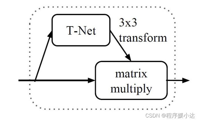
为了保证输入点云的不变性，作者在进行特征提取前先对点云数据进行对齐操作（也就是input transform），对齐操作是通过训练一个小型的网络（也就是上图中的T-Net）来得到转换矩阵，并将之和输入点云数据相乘来实现。

获取该 3*3 的input transform矩阵的python代码实现如下，我做了一些注释，便于大家理解：

class STN3d(nn.Module):def __init__(self, channel):super(STN3d, self).__init__()self.conv1 = torch.nn.Conv1d(channel, 64, 1)self.conv2 = torch.nn.Conv1d(64, 128, 1)self.conv3 = torch.nn.Conv1d(128, 1024, 1)self.fc1 = nn.Linear(1024, 512)self.fc2 = nn.Linear(512, 256)self.fc3 = nn.Linear(256, 9)self.relu = nn.ReLU()self.bn1 = nn.BatchNorm1d(64)self.bn2 = nn.BatchNorm1d(128)self.bn3 = nn.BatchNorm1d(1024)self.bn4 = nn.BatchNorm1d(512)self.bn5 = nn.BatchNorm1d(256)def forward(self, x):batchsize = x.size()[0] # shape (batch_size,3,point_nums)x = F.relu(self.bn1(self.conv1(x))) # shape (batch_size,64,point_nums)x = F.relu(self.bn2(self.conv2(x))) # shape (batch_size,128,point_nums)x = F.relu(self.bn3(self.conv3(x))) # shape (batch_size,1024,point_nums)x = torch.max(x, 2, keepdim=True)[0] # shape (batch_size,1024,1)x = x.view(-1, 1024) # shape (batch_size,1024)x = F.relu(self.bn4(self.fc1(x))) # shape (batch_size,512)x = F.relu(self.bn5(self.fc2(x))) # shape (batch_size,256)x = self.fc3(x) # shape (batch_size,9)iden = Variable(torch.from_numpy(np.array([1, 0, 0, 0, 1, 0, 0, 0, 1]).astype(np.float32))).view(1, 9).repeat(batchsize, 1) # # shape (batch_size,9)if x.is_cuda:iden = iden.cuda()# that's the same thing as adding a diagonal matrix(full 1)x = x + iden # iden means that add the input-selfx = x.view(-1, 3, 3) # shape (batch_size,3,3)return x

这其实在原论文中也提到

The mininetwork itself resembles the big network and is composed by basic modules of point independent feature extraction, max pooling and fully connected layers

3*3的input transform矩阵的获取还是比较简单，这么一套操作下来，这个 input transform矩阵就不是固定的了，它会根据网络的输入动态调整矩阵的权重。

和上面的input transform矩阵的获取方式类似，feature transform的 64*64矩阵获取代码实现如下：

class STNkd(nn.Module):def __init__(self, k=64):super(STNkd, self).__init__()self.conv1 = torch.nn.Conv1d(k, 64, 1)self.conv2 = torch.nn.Conv1d(64, 128, 1)self.conv3 = torch.nn.Conv1d(128, 1024, 1)self.fc1 = nn.Linear(1024, 512)self.fc2 = nn.Linear(512, 256)self.fc3 = nn.Linear(256, k * k)self.relu = nn.ReLU()self.bn1 = nn.BatchNorm1d(64)self.bn2 = nn.BatchNorm1d(128)self.bn3 = nn.BatchNorm1d(1024)self.bn4 = nn.BatchNorm1d(512)self.bn5 = nn.BatchNorm1d(256)self.k = kdef forward(self, x):batchsize = x.size()[0]x = F.relu(self.bn1(self.conv1(x)))x = F.relu(self.bn2(self.conv2(x)))x = F.relu(self.bn3(self.conv3(x)))x = torch.max(x, 2, keepdim=True)[0]x = x.view(-1, 1024)x = F.relu(self.bn4(self.fc1(x)))x = F.relu(self.bn5(self.fc2(x)))x = self.fc3(x)iden = Variable(torch.from_numpy(np.eye(self.k).flatten().astype(np.float32))).view(1, self.k * self.k).repeat(batchsize, 1)if x.is_cuda:iden = iden.cuda()x = x + idenx = x.view(-1, self.k, self.k)return x

值得注意的是，论文中提到

However, transformation matrix in the feature space has much higher dimension than the spatial transform matrix, which greatly increases the difficulty of optimization.

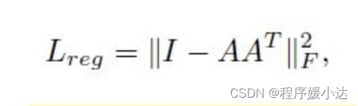
也就是 64*64 的feature transform矩阵很难优化，但是作者发现如果这个矩阵约等于一个正交矩阵，那么优化就方便很多，也稳定很多。为了实现这个矩阵约等于一个正交矩阵，根据正交矩阵的性质，即正交矩阵与其转置的乘积等于单位矩阵。那么作者额外增加了一个损失函数，定义如下：

作者在代码中的实现如下：

def feature_transform_reguliarzer(trans):""" make the transformation matrix of input akin to orthogonal matrix"""d = trans.size()[1]I = torch.eye(d)[None, :, :]if trans.is_cuda:I = I.cuda()loss = torch.mean(torch.norm(torch.bmm(trans, trans.transpose(2, 1) - I), dim=(1, 2)))return loss

至此，有关input transform和feature transform的疑问就解答完毕。

问：为什么做分割任务的时候，输入到分割网络的特征为1088？

这里我们先放上图，如下所示

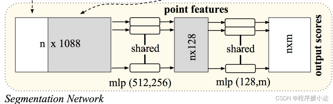
这个 n* 1088 的张量由两部分组成，一个是特征提取网络的输出（大小为n*64 ）,另一个是通过maxpooling后的global feature（大小为1024），在进行两者融合的时候，对global feature进行了广播，那么64+1024就是1088了。为什么要这么做呢？论文中这么提到
After computing the global point cloud feature vector, we feed it back to per point features by concatenating the global feature with each of the point features. Then we extract new per point features based on the combined point features - this time the per point feature is aware of both the local and global information
答案就是作者想要融合点的特征信息（来自特征提取网络的输出）与全局特征（来自global feature）。
问：这一套下来，作者一直在做点之间特征的单独提取，除了最后一层maxpool获取全局信息外，好像并没有将点与其周围点进行融合，提取局部特征呀？

的确，在PointNet这篇文章中确实没有做到像CNN那样逐层提取局部特征。我们知道在CNN中，一个点会与周围若干点进行加权求和（具体取决于卷积核大小），然后获取一个新的点，随着网络层数加深，深层网络的一个点对应原始图像的一个映射区域，这就是感受野的概念。但是本文做的特征提取都是点之间独立进行的，这势必会造成一些问题，至于具体的问题解决，作者在PointNet++展开了说明。（下一篇PointNet++）