在这个实验室中,您将探索评估和改进机器学习模型的技术。

文章目录
- 1 - Packages
- 2-评估学习算法(多项式回归)
- 2.1拆分数据集
- 2.1.1图列、测试集
- 2.2模型评估的误差计算,线性回归
- 2.3比较训练和测试数据的表现
- 3-偏差和方差
- 3.1绘图列、交叉验证、测试
- 3.2寻找最佳阶数
- 3.3调整正则化。
- 3.4获取更多数据:增加训练集大小(m)
- 4-评估学习算法(神经网络)
- 4.1数据集
- 4.2通过计算分类误差来评估分类模型
- 5-模型复杂性
- 5.1复杂模型
- 5.1简单模型
- 6-正则化
- 7-迭代以找到最优正则化值
- 7.1试验
- 祝贺
1 - Packages
首先,让我们运行下面的单元格来导入此分配过程中所需的所有包。
- numpy是科学计算Python的基本包。
- matplotlib是一个流行的Python绘图库。
- scikitslearn是数据挖掘的基本库tensorflow是一个流行的机器学习平台。
import numpy as np
%matplotlib widget
import matplotlib.pyplot as plt
from sklearn.linear_model import LinearRegression, Ridge
from sklearn.preprocessing import StandardScaler, PolynomialFeatures
from sklearn.model_selection import train_test_split
from sklearn.metrics import mean_squared_error
import tensorflow as tf
from tensorflow.keras.models import Sequential
from tensorflow.keras.layers import Dense
from tensorflow.keras.activations import relu,linear
from tensorflow.keras.losses import SparseCategoricalCrossentropy
from tensorflow.keras.optimizers import Adamimport logging
logging.getLogger("tensorflow").setLevel(logging.ERROR)from public_tests_a1 import * tf.keras.backend.set_floatx('float64')
from assigment_utils import *tf.autograph.set_verbosity(0)
2-评估学习算法(多项式回归)
假设你已经创建了一个机器学习模型,你发现它非常适合你的训练数据。你完了吗?不完全是。创建模型的目标是能够预测新示例的值。
在部署新数据之前,如何在新数据上测试模型的性能?
答案有两部分:
- 将原始数据集拆分为“训练”集和“测试”集。
- 使用训练数据来拟合模型的参数
- 使用测试数据在新数据上评估模型
- 开发误差函数来评估模型。
2.1拆分数据集
讲座建议保留20-40%的数据集用于测试。让我们使用sklearn函数train_test_split来执行拆分。运行以下单元格后,请仔细检查形状。
# Generate some data
X,y,x_ideal,y_ideal = gen_data(18, 2, 0.7)
print("X.shape", X.shape, "y.shape", y.shape)#split the data using sklearn routine
X_train, X_test, y_train, y_test = train_test_split(X,y,test_size=0.33, random_state=1)
print("X_train.shape", X_train.shape, "y_train.shape", y_train.shape)
print("X_test.shape", X_test.shape, "y_test.shape", y_test.shape)
import inspect
# 使用 inspect.getsource 获取函数源代码
source_code = inspect.getsource(gen_data)
# 打印函数源代码
print(source_code)
def gen_data(m, seed=1, scale=0.7):""" generate a data set based on a x^2 with added noise """c = 0x_train = np.linspace(0,49,m)np.random.seed(seed)y_ideal = x_train**2 + cy_train = y_ideal + scale * y_ideal*(np.random.sample((m,))-0.5)x_ideal = x_train #for redraw when new data included in Xreturn x_train, y_train, x_ideal, y_ideal
这段代码定义了一个名为
gen_data的函数,其作用如下:
函数功能:
- 生成一个基于 x 2 x^2 x2 函数加入噪声的数据集。
参数说明:
m:数据集中样本的数量。seed:随机种子,用于控制随机数生成过程的随机性。scale:控制噪声的幅度。返回值:
x_train:从0到49均匀分布的m个数据,用作训练集的特征。y_train:根据理想值 x 2 x^2 x2 加上一定比例的随机噪声所生成的目标标签。x_ideal:与x_train相同的理想输入特征,用于在包含新数据时重绘图形。y_ideal:基于 x 2 x^2 x2 函数计算得到的理想目标标签,没有加入噪声。具体操作:
- 首先,生成
x_train,从0到49均匀分布的m个数据点。- 然后,根据随机种子
seed,生成理想目标标签y_ideal,其值为 x 2 x^2 x2。- 接着,在
y_ideal的基础上,添加一定比例的随机噪声,得到最终的训练集目标标签y_train。- 最后,返回生成的特征数据
x_train、目标标签数据y_train、理想特征数据x_ideal和理想目标标签数据y_ideal。这个函数主要用于生成一个带有噪声的数据集,可用于模拟实际情况下的数据。你可以调用这个函数来生成数据集,并用于机器学习模型的训练和测试。如果需要进一步解释或有其他问题,请随时告诉我!我会尽力帮助你。
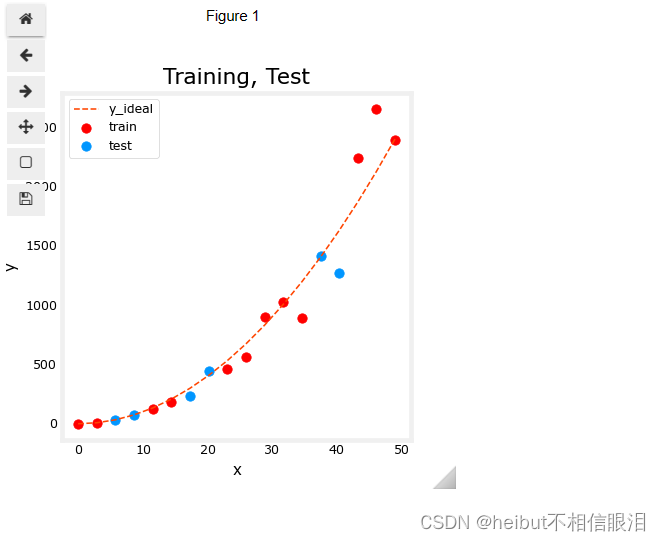
2.1.1图列、测试集
您可以在下面看到,将作为训练一部分的数据点(红色)与未训练模型的数据点混合在一起(测试)。这个特定的数据集是一个添加了噪声的二次函数。所示的“理想”曲线仅供参考。
fig, ax = plt.subplots(1,1,figsize=(4,4))
ax.plot(x_ideal, y_ideal, "--", color = "orangered", label="y_ideal", lw=1)
ax.set_title("Training, Test",fontsize = 14)
ax.set_xlabel("x")
ax.set_ylabel("y")
ax.scatter(X_train, y_train, color = "red",           label="train")
ax.scatter(X_test, y_test,   color = dlc["dlblue"],   label="test")
ax.legend(loc='upper left')
plt.show()
2.2模型评估的误差计算,线性回归
在评估线性回归模型时,将预测值和目标值的误差平方差取平均值。
练习1
下面创建一个函数来评估线性回归模型的数据集上的误差。
# UNQ_C1
# GRADED CELL: eval_mse
def eval_mse(y, yhat):""" Calculate the mean squared error on a data set.Args:y    : (ndarray  Shape (m,) or (m,1))  target value of each exampleyhat : (ndarray  Shape (m,) or (m,1))  predicted value of each exampleReturns:err: (scalar)             """m = len(y)err = 0.0for i in range(m):err_i  = ( (yhat[i] - y[i])**2 ) err   += err_i                                                                err = err / (2*m)                    return(err)
y_hat = np.array([2.4, 4.2])
y_tmp = np.array([2.3, 4.1])
eval_mse(y_hat, y_tmp)
# BEGIN UNIT TEST
test_eval_mse(eval_mse)   #测试目标函数的准确度
# END UNIT TEST
打印函数源代码:
# 使用 inspect.getsource 获取函数源代码
source_code = inspect.getsource(test_eval_mse)# 打印函数源代码
print(source_code)
def test_eval_mse(target):y_hat = np.array([2.4, 4.2])y_tmp = np.array([2.3, 4.1])result = target(y_hat, y_tmp)#assert np.allclose(result, 0.005, atol=1e-6), f"Wrong value. Expected 0.005, got {result}"np.allclose(result, 0.005, atol=1e-6),f"Wrong value. Expected 0.005, got {result}"y_hat = np.array([3.] * 10)y_tmp = np.array([3.] * 10)result = target(y_hat, y_tmp)assert np.allclose(result, 0.), f"Wrong value. Expected 0.0 when y_hat == t_tmp, but got {result}"y_hat = np.array([3.])y_tmp = np.array([0.])result = target(y_hat, y_tmp)assert np.allclose(result, 4.5), f"Wrong value. Expected 4.5, but got {result}. Remember the square termn"y_hat = np.array([3.] * 5)y_tmp = np.array([2.] * 5)result = target(y_hat, y_tmp)assert np.allclose(result, 0.5), f"Wrong value. Expected 0.5, but got {result}. Remember to divide by (2*m)"print("\033[92m All tests passed.")
2.3比较训练和测试数据的表现
让我们建立一个高阶多项式模型来最小化训练误差。这将使用sklearn中的linear_regression函数。如果您想查看详细信息,代码位于导入的实用程序文件中。以下步骤是:
- 创建并拟合模型。(“it”是训练或跑步梯度下降的另一个名称)。
- 计算训练数据的误差。
- 计算测试数据的误差。
# create a model in sklearn, train on training data
degree = 10
lmodel = lin_model(degree)
lmodel.fit(X_train, y_train)# predict on training data, find training error
yhat = lmodel.predict(X_train)
err_train = lmodel.mse(y_train, yhat)# predict on test data, find error
yhat = lmodel.predict(X_test)
err_test = lmodel.mse(y_test, yhat)
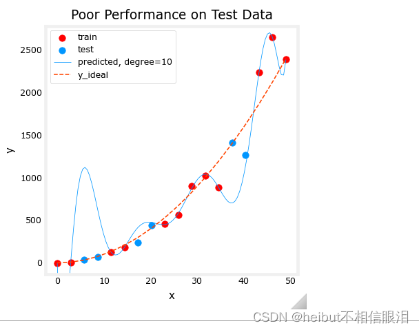
训练集上的计算误差显著小于测试集的计算误差。
print(f"training err {err_train:0.2f}, test err {err_test:0.2f}")
training err 58.01, test err 171215.01
下图显示了为什么会这样。该模型非常适合训练数据。为此,它创建了一个复杂的函数。测试数据不是训练的一部分,模型在预测这些数据方面做得很差。
该模型将被描述为1)过拟合,2)具有高方差,3)“泛化”较差。
# plot predictions over data range
x = np.linspace(0,int(X.max()),100)  # predict values for plot
y_pred = lmodel.predict(x).reshape(-1,1)plt_train_test(X_train, y_train, X_test, y_test, x, y_pred, x_ideal, y_ideal, degree)
测试集错误表明此模型在新数据上无法正常工作。如果你使用测试错误来指导模型的改进,那么模型将在测试数据上表现良好。。。但是测试数据是用来表示新数据的。您还需要另一组数据来测试新的数据性能。
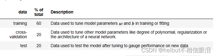
讲座中提出的建议是将数据分为三组。下表所示的训练、交叉验证和测试集的分布是一种典型的分布,但可能会因可用数据量的不同而有所不同。
让我们生成以下三个数据集。我们将再次使用sklearn中的train_test_split,但将调用两次以获得三次拆分:
# Generate  data
X,y, x_ideal,y_ideal = gen_data(40, 5, 0.7)
print("X.shape", X.shape, "y.shape", y.shape)#split the data using sklearn routine
X_train, X_, y_train, y_ = train_test_split(X,y,test_size=0.40, random_state=1)
X_cv, X_test, y_cv, y_test = train_test_split(X_,y_,test_size=0.50, random_state=1)
print("X_train.shape", X_train.shape, "y_train.shape", y_train.shape)
print("X_cv.shape", X_cv.shape, "y_cv.shape", y_cv.shape)
print("X_test.shape", X_test.shape, "y_test.shape", y_test.shape)
X.shape (40,) y.shape (40,)
X_train.shape (24,) y_train.shape (24,)
X_cv.shape (8,) y_cv.shape (8,)
X_test.shape (8,) y_test.shape (8,)
3-偏差和方差
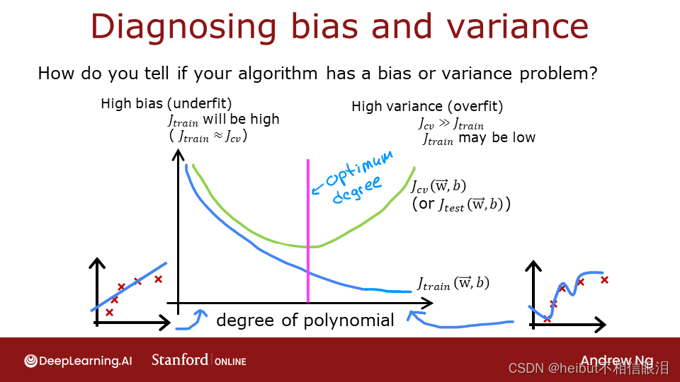
上面,很明显多项式模型的阶数太高了。如何选择好的价值?事实证明,如图所示,训练和交叉验证性能可以提供指导。通过尝试一系列的度值,可以评估训练和交叉验证的性能。随着阶数变得太大,交叉验证性能将开始相对于训练性能下降。让我们在我们的例子中试试这个。
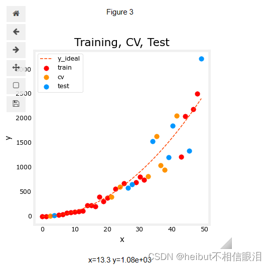
3.1绘图列、交叉验证、测试
您可以在下面看到,将作为训练一部分的数据点(红色)与模型未训练的数据点混合在一起(测试和cv)。
fig, ax = plt.subplots(1,1,figsize=(4,4))
ax.plot(x_ideal, y_ideal, "--", color = "orangered", label="y_ideal", lw=1)
ax.set_title("Training, CV, Test",fontsize = 14)
ax.set_xlabel("x")
ax.set_ylabel("y")ax.scatter(X_train, y_train, color = "red",           label="train")
ax.scatter(X_cv, y_cv,       color = dlc["dlorange"], label="cv")
ax.scatter(X_test, y_test,   color = dlc["dlblue"],   label="test")
ax.legend(loc='upper left')
plt.show()
3.2寻找最佳阶数
在之前的实验室中,您发现可以通过使用多项式来创建能够拟合复杂曲线的模型(请参阅课程1,第2周“特征工程和多项式回归实验室”)。此外,您证明了通过增加多项式的次数,可以创建过拟合。(参见课程1,第3周,过度拟合实验室)。让我们用这些知识来测试我们区分过度拟合和欠拟合的能力。
让我们反复训练模型,每次迭代都增加多项式的次数。在这里,我们将使用scikit-learn线性回归模型来提高速度和简单性。
max_degree = 9
err_train = np.zeros(max_degree)
err_cv = np.zeros(max_degree)
x = np.linspace(0,int(X.max()),100)
y_pred = np.zeros((100,max_degree))  #columns are lines to plotfor degree in range(max_degree):lmodel = lin_model(degree+1)lmodel.fit(X_train, y_train)yhat = lmodel.predict(X_train)err_train[degree] = lmodel.mse(y_train, yhat)yhat = lmodel.predict(X_cv)err_cv[degree] = lmodel.mse(y_cv, yhat)y_pred[:,degree] = lmodel.predict(x)optimal_degree = np.argmin(err_cv)+1  #这行代码的作用是找到交叉验证误差(cross-validation error)数组 err_cv 中的最小值,并返回最小值所对应的索引加一(因为索引是从0开始的,所以要加一),即找到最优的多项式回归模型的阶数。
让我们画出结果:
plt.close("all") # 用于关闭所有当前打开的 Matplotlib 图形窗口,以便开始绘制新的图表或清理当前的图形环境。
plt_optimal_degree(X_train, y_train, X_cv, y_cv, x, y_pred, x_ideal, y_ideal, err_train, err_cv, optimal_degree, max_degree)
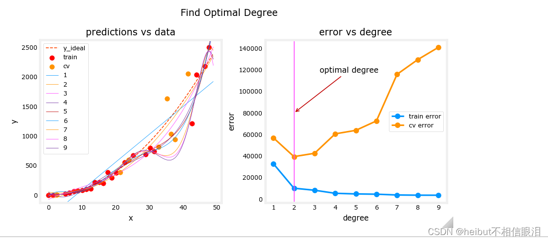
上图表明,将数据分为两组,即模型训练的数据和模型未训练的数据,可用于确定模型是否拟合不足或拟合过度。在我们的例子中,我们通过增加所使用的多项式的次数,创建了从欠拟合到过拟合的各种模型。
- 在左图中,实线表示这些模型的预测。次数为1的多项式模型生成一条与极少数数据点相交的直线,而最大次数则与每个数据点非常接近。
- 右侧:
- 训练数据上的误差(蓝色)随着模型复杂度的增加而减小,正如预期的那样。
- 交叉验证数据的误差最初随着模型开始与数据一致而减小,但随后随着模型开始在训练数据上过度拟合而增大(未能泛化)。
值得注意的是,这些例子中的曲线并不像你在课堂上画的那样平滑。很明显,分配给每组的特定数据点会显著改变您的结果。总的趋势才是最重要的。
3.3调整正则化。
在以前的实验室中,您已经使用正则化来减少过拟合。类似于阶数,可以使用相同的方法来调整正则化参数lambda(𝜆).
让我们通过从一个高阶多项式开始并改变正则化参数来证明这一点。
lambda_range = np.array([0.0, 1e-6, 1e-5, 1e-4,1e-3,1e-2, 1e-1,1,10,100])
num_steps = len(lambda_range)
degree = 10
err_train = np.zeros(num_steps)
err_cv = np.zeros(num_steps)
x = np.linspace(0,int(X.max()),100)
y_pred = np.zeros((100,num_steps))  #columns are lines to plotfor i in range(num_steps):lambda_= lambda_range[i]lmodel = lin_model(degree, regularization=True, lambda_=lambda_)lmodel.fit(X_train, y_train)yhat = lmodel.predict(X_train)err_train[i] = lmodel.mse(y_train, yhat)yhat = lmodel.predict(X_cv)err_cv[i] = lmodel.mse(y_cv, yhat)y_pred[:,i] = lmodel.predict(x)optimal_reg_idx = np.argmin(err_cv)
plt.close("all")
plt_tune_regularization(X_train, y_train, X_cv, y_cv, x, y_pred, err_train, err_cv, optimal_reg_idx, lambda_range)
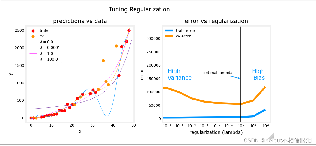
上图显示,随着正则化的增加,模型从高方差(过拟合)模型转变为高偏差(欠拟合)模型。右图中的垂直线显示了lambda的最佳值。在这个例子中,多项式次数被设置为10。
3.4获取更多数据:增加训练集大小(m)
当模型过拟合(高方差)时,收集额外的数据可以提高性能。让我们在这里试试。
X_train, y_train, X_cv, y_cv, x, y_pred, err_train, err_cv, m_range,degree = tune_m()
plt_tune_m(X_train, y_train, X_cv, y_cv, x, y_pred, err_train, err_cv, m_range, degree)
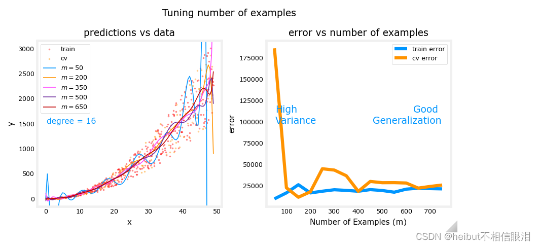
上面的图显示,当模型具有高方差且过拟合时,添加更多的示例可以提高性能。注意左图中的曲线。具有最高值的最终曲线𝑚是位于数据中心的平滑曲线。在右边,随着示例数量的增加,训练集和交叉验证集的性能收敛到相似的值。请注意,曲线并不像你在课堂上看到的那样平滑。这是意料之中的事。趋势仍然很明显:更多的数据可以提高泛化能力。
请注意,当模型具有高偏差(底部配合)时添加更多示例并不能提高性能。
显示tune_m()
# 使用 inspect.getsource 获取函数源代码
source_code = inspect.getsource(tune_m)
# 打印函数源代码
print(source_code)
def tune_m():""" tune the number of examples to reduce overfitting """m = 50m_range = np.array(m*np.arange(1,16))num_steps = m_range.shape[0]degree = 16err_train = np.zeros(num_steps) err_cv = np.zeros(num_steps) y_pred = np.zeros((100,num_steps)) for i in range(num_steps):X, y, y_ideal, x_ideal = gen_data(m_range[i],5,0.7)x = np.linspace(0,int(X.max()),100) X_train, X_, y_train, y_ = train_test_split(X,y,test_size=0.40, random_state=1)X_cv, X_test, y_cv, y_test = train_test_split(X_,y_,test_size=0.50, random_state=1)lmodel = lin_model(degree) # no regularizationlmodel.fit(X_train, y_train)yhat = lmodel.predict(X_train)err_train[i] = lmodel.mse(y_train, yhat)yhat = lmodel.predict(X_cv)err_cv[i] = lmodel.mse(y_cv, yhat)y_pred[:,i] = lmodel.predict(x)return(X_train, y_train, X_cv, y_cv, x, y_pred, err_train, err_cv, m_range,degree)4-评估学习算法(神经网络)
上面,您调整了多项式回归模型的各个方面。在这里,您将使用一个神经网络模型。让我们从创建一个分类数据集开始。
4.1数据集
运行下面的单元格以生成数据集,并将其拆分为训练集、交叉验证集和测试集。在本例中,我们增加了交叉验证数据点的百分比以进行强调。
# Generate and split data set
X, y, centers, classes, std = gen_blobs()
# split the data. Large CV population for demonstration
X_train, X_, y_train, y_ = train_test_split(X,y,test_size=0.50, random_state=1)
X_cv, X_test, y_cv, y_test = train_test_split(X_,y_,test_size=0.20, random_state=1)
print("X_train.shape:", X_train.shape, "X_cv.shape:", X_cv.shape, "X_test.shape:", X_test.shape)
X_train.shape: (400, 2) X_cv.shape: (320, 2) X_test.shape: (80, 2)
显示gen_blobs():
# 使用 inspect.getsource 获取函数源代码
source_code = inspect.getsource(gen_blobs)
# 打印函数源代码
print(source_code)
def gen_blobs():classes = 6m = 800std = 0.4centers = np.array([[-1, 0], [1, 0], [0, 1], [0, -1], [-2,1],[-2,-1]])X, y = make_blobs(n_samples=m, centers=centers, cluster_std=std, random_state=2, n_features=2)return (X, y, centers, classes, std)plt_train_eq_dist(X_train, y_train,classes, X_cv, y_cv, centers, std)
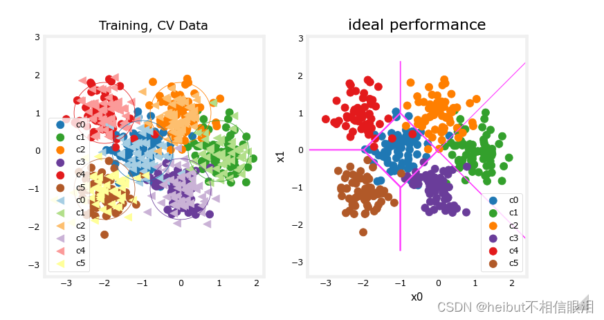
在上面,您可以看到左侧的数据。有六个按颜色识别的簇。显示了训练点(点)和交叉验证点(三角形)。有趣的是那些位于模糊位置的点,其中任何一个集群都可能认为它们是成员。你希望神经网络模型能做什么?什么是过度拟合的例子?填充不足?
右边是一个“理想”模型的例子,或者一个知道数据来源的人可能创建的模型。这些线表示中心点之间距离相等的“等距离”边界。值得注意的是,该模型会对大约8%的总数据集进行“错误分类”。
4.2通过计算分类误差来评估分类模型
这里使用的分类模型的评估函数只是错误预测的分数:
练习2
下面,完成计算分类错误的例程。注意,在这个实验室中,目标值是类别的索引,而不是热编码的。
# UNQ_C2
# GRADED CELL: eval_cat_err
def eval_cat_err(y, yhat):""" Calculate the categorization errorArgs:y    : (ndarray  Shape (m,) or (m,1))  target value of each exampleyhat : (ndarray  Shape (m,) or (m,1))  predicted value of each exampleReturns:|cerr: (scalar)             """m = len(y)incorrect = 0for i in range(m):if yhat[i] != y[i]:    # @REPLACEincorrect += 1     # @REPLACEcerr = incorrect/m         # @REPLACEreturn(cerr)
y_hat = np.array([1, 2, 0])
y_tmp = np.array([1, 2, 3])
print(f"categorization error {np.squeeze(eval_cat_err(y_hat, y_tmp)):0.3f}, expected:0.333" )
y_hat = np.array([[1], [2], [0], [3]])
y_tmp = np.array([[1], [2], [1], [3]])
print(f"categorization error {np.squeeze(eval_cat_err(y_hat, y_tmp)):0.3f}, expected:0.250" )# BEGIN UNIT TEST
test_eval_cat_err(eval_cat_err)
# END UNIT TEST
# BEGIN UNIT TEST
test_eval_cat_err(eval_cat_err)
# END UNIT TEST
categorization error 0.333, expected:0.333
categorization error 0.250, expected:0.250All tests passed.All tests passed.
5-模型复杂性
下面,您将构建两个模型。一个复杂的模型和一个简单的模型。您将评估模型,以确定它们是否可能过拟合或欠拟合。
5.1复杂模型
练习3
下面,组成一个三层模型:
- 具有120个单元的致密层,relu激活
- 具有40个单元的稠密层,relu-activation
- 具有6个单元的密集层和线性激活(非softmax)
- 使用损失与稀疏类别交叉熵进行编译,记住使用from_logits=True Adam优化器,学习率为0.01。
# UNQ_C3
# GRADED CELL: model
import logging
logging.getLogger("tensorflow").setLevel(logging.ERROR)tf.random.set_seed(1234)
model = Sequential([Dense(120, activation = 'relu', name = "L1"),      Dense(40, activation = 'relu', name = "L2"),         Dense(classes, activation = 'linear', name = "L3")  ], name="Complex"
)
model.compile(loss=tf.keras.losses.SparseCategoricalCrossentropy(from_logits=True),          optimizer=tf.keras.optimizers.Adam(0.01),
)
# BEGIN UNIT TEST
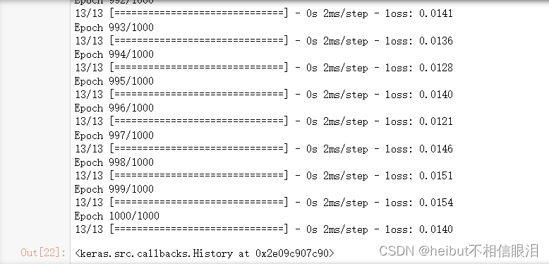
model.fit(X_train, y_train,epochs=1000
)
# END UNIT TEST
在机器学习中,epochs 是指将整个数据集在神经网络中训练一次的次数。具体来说,在神经网络的训练过程中,数据集会被分成若干个批次(batches),每次迭代(iteration)神经网络会接收一个批次的数据进行前向传播和反向传播来更新模型的参数。而完成对整个数据集的一次遍历就称为一个 epoch。
# BEGIN UNIT TEST
model.summary()
model_test(model, classes, X_train.shape[1])
# END UNIT TEST
Model: "Complex"
_________________________________________________________________Layer (type)                Output Shape              Param #
=================================================================L1 (Dense)                  (None, 120)               360       L2 (Dense)                  (None, 40)                4840      L3 (Dense)                  (None, 6)                 246       =================================================================
Total params: 5446 (42.55 KB)
Trainable params: 5446 (42.55 KB)
Non-trainable params: 0 (0.00 Byte)
_________________________________________________________________
All tests passed!
#make a model for plotting routines to call
model_predict = lambda Xl: np.argmax(tf.nn.softmax(model.predict(Xl)).numpy(),axis=1)
plt_nn(model_predict,X_train,y_train, classes, X_cv, y_cv, suptitle="Complex Model")
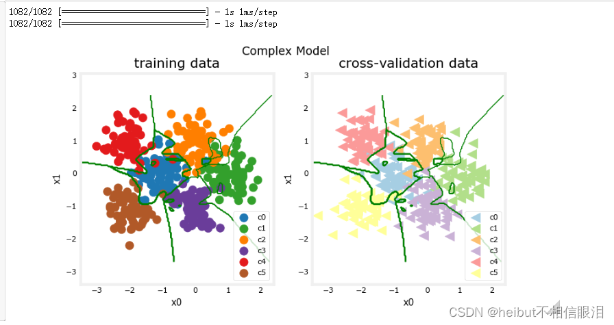
这个模型非常努力地捕捉每个类别的异常值。因此,它对一些交叉验证数据进行了错误分类。让我们计算一下分类误差。
training_cerr_complex = eval_cat_err(y_train, model_predict(X_train))
cv_cerr_complex = eval_cat_err(y_cv, model_predict(X_cv))
print(f"categorization error, training, complex model: {training_cerr_complex:0.3f}")
print(f"categorization error, cv,       complex model: {cv_cerr_complex:0.3f}")
13/13 [==============================] - 0s 2ms/step
10/10 [==============================] - 0s 1ms/step
categorization error, training, complex model: 0.005
categorization error, cv,       complex model: 0.109
5.1简单模型
现在,让我们尝试一个简单的模型
练习4
下面,组成一个两层模型:
- 具有6个单元的致密层,relu激活
- 具有6个单位的致密层和线性激活
- 使用损失SparseCategoricalCrossentropy编译,记住使用from_logits=True
Adam优化器,学习率为0.01。
# UNQ_C4
# GRADED CELL: model_stf.random.set_seed(1234)
model_s = Sequential([Dense(6, activation = 'relu', name="L1"),            # @REPLACEDense(classes, activation = 'linear', name="L2")     # @REPLACE], name = "Simple"
)
model_s.compile(loss=tf.keras.losses.SparseCategoricalCrossentropy(from_logits=True),     # @REPLACEoptimizer=tf.keras.optimizers.Adam(0.01),     # @REPLACE
)
import logging
logging.getLogger("tensorflow").setLevel(logging.ERROR)# BEGIN UNIT TEST
model_s.fit(X_train,y_train,epochs=1000
)
# END UNIT TEST
# BEGIN UNIT TEST
model_s.summary()model_s_test(model_s, classes, X_train.shape[1])
# END UNIT TEST
Model: "Simple"
_________________________________________________________________Layer (type)                Output Shape              Param #
=================================================================L1 (Dense)                  (None, 6)                 18        L2 (Dense)                  (None, 6)                 42        =================================================================
Total params: 60 (480.00 Byte)
Trainable params: 60 (480.00 Byte)
Non-trainable params: 0 (0.00 Byte)
_________________________________________________________________
All tests passed!
#make a model for plotting routines to call
model_predict_s = lambda Xl: np.argmax(tf.nn.softmax(model_s.predict(Xl)).numpy(),axis=1)
plt_nn(model_predict_s,X_train,y_train, classes, X_cv, y_cv, suptitle="Simple Model")
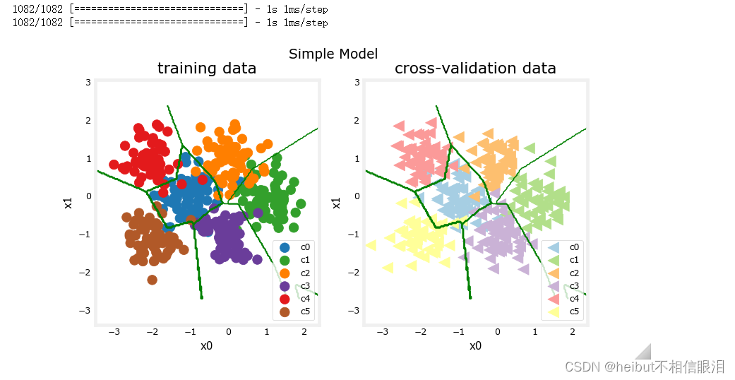
这个简单的模型做得很好。让我们计算一下分类误差。
training_cerr_simple = eval_cat_err(y_train, model_predict_s(X_train))
cv_cerr_simple = eval_cat_err(y_cv, model_predict_s(X_cv))
print(f"categorization error, training, simple model, {training_cerr_simple:0.3f}, complex model: {training_cerr_complex:0.3f}" )
print(f"categorization error, cv,       simple model, {cv_cerr_simple:0.3f}, complex model: {cv_cerr_complex:0.3f}" )
13/13 [==============================] - 0s 1ms/step
10/10 [==============================] - 0s 1ms/step
categorization error, training, simple model, 0.060, complex model: 0.005
categorization error, cv,       simple model, 0.081, complex model: 0.109
我们的简单模型在训练数据上有更高的分类误差,但在交叉验证数据上比更复杂的模型做得更好。
6-正则化
与多项式回归的情况一样,可以应用正则化来缓和更复杂模型的影响。让我们在下面试试这个。
练习5
重建你的复杂模型,但这次包括正则化。下面,组成一个三层模型:
- 具有120个单元的致密层,relu活化,kernel_regularizer=tf.keras.regularizer.l2(0.1)
- 具有40个单元的稠密层,relu-活化,kernel_regularifier=tf.karas.regulariser.l2(0.1)
- 具有6个单元和线性活化的致密层。
- 使用损失SparseCategoricalCrossentropy编译,记住使用from_logits=True
Adam优化器,学习率为0.01。
# UNQ_C5
# GRADED CELL: model_rtf.random.set_seed(1234)
model_r = Sequential([Dense(120, activation = 'relu', kernel_regularizer=tf.keras.regularizers.l2(0.1), name="L1"), Dense(40, activation = 'relu', kernel_regularizer=tf.keras.regularizers.l2(0.1), name="L2"),  Dense(classes, activation = 'linear', name="L3")  ], name="ComplexRegularized"
)
model_r.compile(loss=tf.keras.losses.SparseCategoricalCrossentropy(from_logits=True), optimizer=tf.keras.optimizers.Adam(0.01),
)
# BEGIN UNIT TEST
model_r.fit(X_train, y_train,epochs=1000
)
# END UNIT TEST

# BEGIN UNIT TEST
model_r.summary()model_r_test(model_r, classes, X_train.shape[1])
# END UNIT TEST
Model: "ComplexRegularized"
_________________________________________________________________Layer (type)                Output Shape              Param #
=================================================================L1 (Dense)                  (None, 120)               360       L2 (Dense)                  (None, 40)                4840      L3 (Dense)                  (None, 6)                 246       =================================================================
Total params: 5446 (42.55 KB)
Trainable params: 5446 (42.55 KB)
Non-trainable params: 0 (0.00 Byte)
_________________________________________________________________
ddd
All tests passed!
#make a model for plotting routines to call
model_predict_r = lambda Xl: np.argmax(tf.nn.softmax(model_r.predict(Xl)).numpy(),axis=1)plt_nn(model_predict_r, X_train,y_train, classes, X_cv, y_cv, suptitle="Regularized")
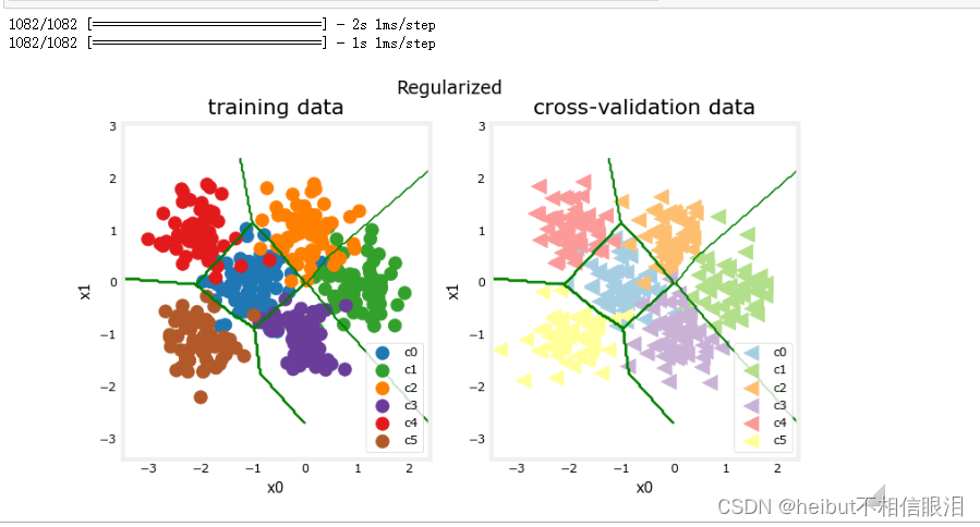
结果看起来与“理想”模型非常相似。让我们检查一下分类错误。
training_cerr_reg = eval_cat_err(y_train, model_predict_r(X_train))
cv_cerr_reg = eval_cat_err(y_cv, model_predict_r(X_cv))
test_cerr_reg = eval_cat_err(y_test, model_predict_r(X_test))
print(f"categorization error, training, regularized: {training_cerr_reg:0.3f}, simple model, {training_cerr_simple:0.3f}, complex model: {training_cerr_complex:0.3f}" )
print(f"categorization error, cv,       regularized: {cv_cerr_reg:0.3f}, simple model, {cv_cerr_simple:0.3f}, complex model: {cv_cerr_complex:0.3f}" )
13/13 [==============================] - 0s 1ms/step
10/10 [==============================] - 0s 1ms/step
3/3 [==============================] - 0s 2ms/step
categorization error, training, regularized: 0.062, simple model, 0.060, complex model: 0.005
categorization error, cv,       regularized: 0.056, simple model, 0.081, complex model: 0.109
简单模型在训练集中比正则化模型好一点,但在交叉验证集中较差。
7-迭代以找到最优正则化值
正如您在线性回归中所做的那样,您可以尝试许多正则化值。运行此代码需要几分钟时间。如果你有时间,你可以运行它并检查结果。如果没有,你已经完成了作业的评分部分!
tf.random.set_seed(1234)
lambdas = [0.0, 0.001, 0.01, 0.05, 0.1, 0.2, 0.3]
models=[None] * len(lambdas)
for i in range(len(lambdas)):lambda_ = lambdas[i]models[i] =  Sequential([Dense(120, activation = 'relu', kernel_regularizer=tf.keras.regularizers.l2(lambda_)),Dense(40, activation = 'relu', kernel_regularizer=tf.keras.regularizers.l2(lambda_)),Dense(classes, activation = 'linear')])models[i].compile(loss=tf.keras.losses.SparseCategoricalCrossentropy(from_logits=True),optimizer=tf.keras.optimizers.Adam(0.01),)models[i].fit(X_train,y_train,epochs=1000)print(f"Finished lambda = {lambda_}")
plot_iterate(lambdas, models, X_train, y_train, X_cv, y_cv)
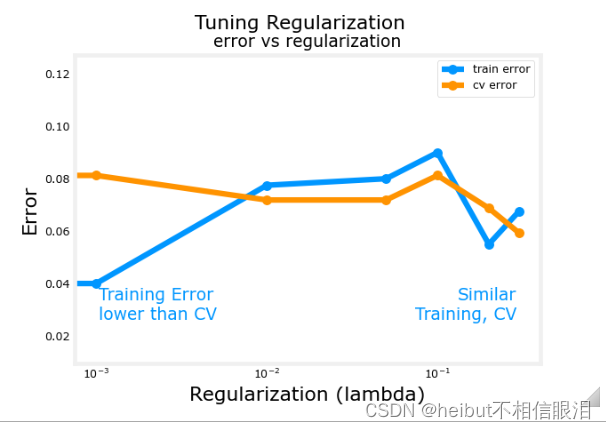
随着正则化程度的提高,模型在训练和交叉验证数据集上的性能趋于收敛。对于该数据集和模型,λ>0.01似乎是一个合理的选择。
7.1试验
让我们在测试集上尝试我们的优化模型,并将其与“理想”性能进行比较。
plt_compare(X_test,y_test, classes, model_predict_s, model_predict_r, centers)

我们的测试集很小,似乎有很多异常值,所以分类误差很高。然而,我们优化模型的性能与理想性能相当。
祝贺
在评估机器学习模型时,您已经熟悉了要应用的重要工具。即
- 将数据分为经过训练的和未经过训练的数据集可以区分欠拟合和过拟合
- 创建三个数据集,“训练”、“交叉验证”和“测试”
- 可以训练参数𝑊,𝐵
- 使用训练集调整模型参数,如复杂性、正则化和交叉验证集的示例数量,使用测试集评估您的“真实世界”性能。
- 比较训练与交叉验证的性能可以深入了解模型的过拟合(高方差)或欠拟合(高偏差)倾向