ajax不利于seo
Lately, my parents will often bring up in conversation their desire to move away from their California home and find a new place to settle down for retirement. Typically they will cite factors that they perceive as having altered the essence of their suburban and rural county such as higher costs of living, population growth, worsening traffic, and growing rates of violent crime that they say have made them feel estranged from their community in recent years. Despite these concerns, both admit that there is much they would miss about their current home such as the mild climate of the California coast, the abundant natural beauty of the region, and an vast matrix of open space and public lands that allow them to enjoy outdoor hobbies throughout the year.
最近,我的父母经常会谈论他们想离开加利福尼亚州的家,并找到一个定居下来退休的新地方的愿望。 通常,他们会引用自己认为改变了郊区和乡村县城本质的因素,例如更高的生活成本,人口增长,交通状况恶化以及暴力犯罪率上升,他们说这使他们对自己的社区感到疏远。最近几年。 尽管存在这些担忧,但他们俩都承认,他们目前的住所会遗漏很多东西,例如加利福尼亚海岸的温和气候,该地区丰富的自然风光以及广阔的开放空间和公共土地,使他们能够享受全年都有户外活动。
The idea for Niche came from wanting to help my parents explore their relocation options by taking into consideration what matters most to them about the place they live now. The name of this app is taken from a foundational concept in biology. While many definitions of a niche exist, from verbal models to mathematical frameworks, virtually all definitions agree that one’s niche can be thought of as the set of environmental conditions necessary for an organism to thrive. While some species can only tolerate a narrow range of conditions (think temperature, light, salinity, etc.) others will do just fine when exposed to large changes in these same variables. But even members of the same species will occupy a different niche due to the individual variation that exists in their anatomy, physiology, and behavior. The point is that no two individuals experience a shared environment in exactly the same way. We all have different tolerances.
Niche的想法来自希望通过考虑父母对他们现在住的地方最重要的问题来帮助我的父母探索他们的搬迁选择。 该应用程序的名称来自生物学的基本概念。 尽管存在许多关于生态位的定义,从语言模型到数学框架,但几乎所有定义都同意,人们的生态位可以被认为是有机体赖以生存的一系列环境条件。 虽然某些物种只能忍受狭窄的条件(例如温度,光照,盐度等),但其他物种在暴露于这些相同变量的较大变化时也可以正常工作。 但是,即使是同一物种的成员,由于其解剖结构,生理和行为方面的个体差异,它们也会占据不同的位置。 关键是,没有两个人会以完全相同的方式体验共享的环境。 我们都有不同的容忍度。
Borrowing from this concept, it is easy to imagine how our own ability to thrive will be influenced by our surroundings. Niche works by asking users to identify a location where they would like to live and answer a few questions about what is important to them about that place. The program then identifies other areas in the country with similar features before making recommendations on relocation options. Niche considers both the more salient characteristics of a location such as the climate and land uses as well as factors that may be less conspicuous such as economic, demographic, and political indicators. Niche relies on the belief that the best tools to guide our understanding of the conditions best suit us as individuals will come from reflecting on our experiences. You know what you want to find in the places you want to live and Niche can help you find them.
从这个概念中借用,很容易想象我们的生存能力将受到周围环境的影响。 Niche的工作原理是要求用户确定他们想要居住的位置,并回答一些有关该位置对他们而言重要的问题。 然后,该程序在建议搬迁选项之前,先确定该国其他具有类似特征的地区。 Niche既考虑了地理位置的突出特征,例如气候和土地利用,也考虑了经济,人口和政治指标等不太明显的因素。 Niche依靠这样一种信念,即指导个人对条件的理解的最佳工具最适合我们,因为个人会从反思我们的经验中获得。 您知道要在自己想住的地方找到什么,Niche可以帮助您找到它们。
All of the data preparation and analysis was performed using R because I knew that I would create the interactive front-end with Shiny. Below, I detail the data and methods that went into creating Niche, but do not cover what went into creating the Shiny app. If you would like to know more about that, you can find that code as well as the rest of the project source code on my GitHub repository. If you have any feedback, questions, or suggestions please get in touch with me by email.
所有数据准备和分析都是使用R进行的,因为我知道我将使用Shiny创建交互式前端。 下面,我详细介绍创建Niche所需的数据和方法,但不介绍创建Shiny应用程序所需的内容。 如果您想了解更多信息,可以在我的GitHub存储库中找到该代码以及项目源代码的其余部分。 如果您有任何反馈,问题或建议,请通过电子邮件与我联系 。
0.获取县级边界数据,此分析的单位 (0. Get County-level Boundary Data, the unit of this analysis)
Before getting started, I needed to aquire a geospatial dataset for all of the counties in the contiguous 48 U.S. states. Fortunately, ggplot2 packages makes this easy with the ggplot2::map_data() function. However, I knew that I would eventually like to have the data as an ‘sf’ type object used by the sf (“simple features”) geospatial package. Therefore, I had to first download the county level data using ggplot2, convert the coordinate data into a ’Spatial*’ object (used by the sp package), save this data to local storage as a shapefile, and finally read the file back into R using sf::st_read(). I decided to save the data as a shapefile as an intermediate data prodcut because the conversion to ‘SpatialPolygonsDataFrame’ was non-trivial (this code helped) and took a bit of time to finish.
开始之前,我需要获取美国48个连续州的所有县的地理空间数据集。 幸运的是, ggplot2软件包通过ggplot2::map_data()函数使此操作变得容易。 但是,我知道我最终希望将数据作为sf (“简单要素”)地理空间包使用的“ sf”类型对象。 因此,我必须首先使用ggplot2下载县级数据,将坐标数据转换为“ Spatial *”对象(由sp程序包使用),然后将此数据作为shapefile保存到本地存储中,最后将文件读回到R使用sf::st_read() 。 我决定将数据另存为shapefile作为中间数据产品,因为到“ SpatialPolygonsDataFrame”的转换非常简单( 此代码有所帮助 ),并且花费了一些时间才能完成。
library(ggplot2)
county_df <- map_data("county") %>%
  mutate(region = tolower(region)) %>%
  mutate(subregion = tolower(subregion)) %>%
  mutate(subregion = str_replace(subregion, "st ", "saint ")) %>%
  mutate(subregion = str_replace(subregion, "ste ", "saint ")) %>%
  mutate(region = str_replace(region, "\\s", "_")) %>%
  mutate(subregion = str_replace(subregion, "\\s", "_")) %>%
  mutate(id = paste(subregion, region, sep=",_"))
coordinates(county_df) = c("long","lat") #converts to SpatialPointsDataFrame
#convert to SpatialPolygonsDataFrame
#https://stackoverflow.com/questions/21759134/convert-spatialpointsdataframe-to-spatialpolygons-in-r
points2polygons <- function(df,data) {
  get.grpPoly <- function(group,ID,df) {
    Polygon(coordinates(df[df$id==ID & df$group==group,]))
  }
  get.spPoly  <- function(ID,df) {
    Polygons(lapply(unique(df[df$id==ID,]$group),get.grpPoly,ID,df),ID)
  }
  spPolygons  <- SpatialPolygons(lapply(unique(df$id),get.spPoly,df))
  SpatialPolygonsDataFrame(spPolygons,match.ID=T,data=data)
}
sp_dat = county_df$id %>%
  unique() %>%
  factor() %>%
  data.frame(name=.)
rownames(sp_dat) = sp_dat$name
sp_dat$id = as.numeric(sp_dat$name)
counties <- points2polygons(county_df, sp_dat) #this may take a moment
locs = counties$name %>%
  as.character() %>%
  strsplit(split = ",_") %>%
  do.call("rbind", .)
counties$county = locs[,1]
counties$state = locs[,2]
Once completed, I had a map of the United States composed of polygons for each county. Now, any new columns added to d (an ‘sf’ object) will be automatically georeferenced.
完成后,我将获得一个由每个县的多边形组成的美国地图。 现在,添加到d (“ sf”对象)的所有新列都将自动进行地理参考。
d <- st_read("raw_data/shape/counties.shp", quiet = TRUE)
st_crs(d) <- CRS("+proj=longlat")
print(d$geometry)## Geometry set for 3076 features
## geometry type:  MULTIPOLYGON
## dimension:      XY
## bbox:           xmin: -124.6813 ymin: 25.12993 xmax: -67.00742 ymax: 49.38323
## CRS:            +proj=longlat +ellps=WGS84
## First 5 geometries:
## MULTIPOLYGON (((-86.50517 32.3492, -86.53382 32...
## MULTIPOLYGON (((-87.93757 31.14599, -87.93183 3...
## MULTIPOLYGON (((-85.42801 31.61581, -85.74313 3...
## MULTIPOLYGON (((-87.02083 32.83621, -87.30731 3...
## MULTIPOLYGON (((-86.9578 33.8618, -86.94062 33....d %>%
  ggplot() +
    theme_minimal() +
    geom_sf(fill="steelblue", color="white", size=0.1)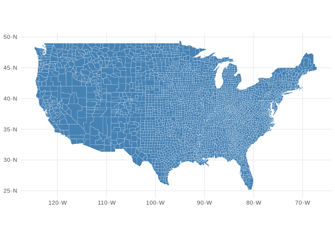
1. WorldClim的气候变量 (1. Climatic Variables from WorldClim)
To characterize the climatic conditions for each county, I turned to WorldClim’s global climate database, specifically their ‘bioclim’ collection of annual climate summary measurements. As with the county-level polygons, there exists an API for downloading these files directly from R, this time using the raster::getData() function. Below is the code for downloading ‘bioclim’ data at a resolution of 5 arc minutes, or approximately 64 km² per grid cell at the latitudes considered here.
为了描述每个县的气候条件,我求助于WorldClim的全球气候数据库,特别是他们的“ bioclim”年度气候摘要测量值集合。 与县级多边形一样,有一个API可直接从R下载这些文件,这次使用raster::getData()函数。 以下是在此处考虑的纬度下,以5弧分钟的分辨率或每个网格单元大约64km²的分辨率下载“ bioclim”数据的代码。
##Download environmental variables
getData('worldclim', var='bio', res=2.5, path = "raw_data/") #123 MB download
varsToGet = c("tmean","tmin","tmax","prec","bio","alt")
sapply(varsToGet, function(x) getData(name = "worldclim", download = TRUE, res=10, var=x))#bioclim variables (https://worldclim.org/raw_data/bioclim.html)
# BIO1 = Annual Mean Temperature
# BIO2 = Mean Diurnal Range (Mean of monthly (max temp - min temp))
# BIO3 = Isothermality (BIO2/BIO7) (×100)
# BIO4 = Temperature Seasonality (standard deviation × 100)
# BIO5 = Max Temperature of Warmest Month
# BIO6 = Min Temperature of Coldest Month
# BIO7 = Temperature Annual Range (BIO5-BIO6)
# BIO8 = Mean Temperature of Wettest Quarter
# BIO9 = Mean Temperature of Driest Quarter
# BIO10 = Mean Temperature of Warmest Quarter
# BIO11 = Mean Temperature of Coldest Quarter
# BIO12 = Annual Precipitation
# BIO13 = Precipitation of Wettest Month
# BIO14 = Precipitation of Driest Month
# BIO15 = Precipitation Seasonality (Coefficient of Variation)
# BIO16 = Precipitation of Wettest Quarter
# BIO17 = Precipitation of Driest Quarter
# BIO18 = Precipitation of Warmest Quarter
# BIO19 = Precipitation of Coldest Quarter
With the raw climate data saved to a local directy, the *.bil files are identified, sorted by name, and queued for import back into the R environment.
将原始气候数据保存到本地目录后,*。bil文件被标识,按名称排序,并排队等待导入回到R环境中。
bclimFiles = list.files("raw_data/wc5/", pattern = "bio", full.names = TRUE)[-1]
bclimFiles = bclimFiles[str_detect(bclimFiles, "bil")==TRUE]
orderFiles = str_extract_all(bclimFiles, pattern="[[:digit:]]+") %>%
  do.call("rbind",.) %>%
  as.matrix %>%
  apply(., 2, as.numeric)
orderFiles = order(orderFiles[,2])
bioclim = stack(bclimFiles[orderFiles]) %>%
  crop(., extent(d) + c(-1,1) + 2)plot(bioclim, col=viridis::viridis(15))
Feature extraction using principal components analysis
使用主成分分析进行特征提取
The dataset includes 19 variables but deal mostly with characterizing temperature and precipitation patterns. As a result, we might expect that many of these variables will be highly correlated with one another, and would want to consider using feature extraction to distill the variation to fewer dimensions.
该数据集包括19个变量,但主要处理特征温度和降水模式。 结果,我们可能期望其中许多变量彼此高度相关,并希望考虑使用特征提取将变化提炼为更少的维度。
Indeed what I have chosen to do here is perform principal components analysis (PCA) on the climate data in order to collapse raw variables into a smaller number of axes. Before I did that, however, it was important to first normalize each variable by centering each around its mean and re-scaling the variance to 1 by dividing measurements by their standard deviation. After processing the data and performing the PCA, I found that approximately 85% of the total variation could was captured by the first four principal components, and chose to hold onto these axes of variation in order to characterize climatic variation in the data set.
确实,我在这里选择做的是对气候数据执行主成分分析(PCA),以将原始变量分解为较少数量的轴。 但是,在执行此操作之前,重要的是首先通过将每个变量均值居中并将每个变量除以标准差将其重新标定为1来对每个变量进行归一化。 在处理了数据并执行了PCA之后,我发现前四个主要成分可以捕获大约85%的总变化,并选择保留这些变化轴以表征数据集中的气候变化。
#normalize data to mean 0 and unit variance
normalize <- function(x){
  mu <- mean(x, na.rm=TRUE)
  sigma <- sd(x, na.rm=TRUE)
  y <- (x-mu)/sigma
  return(y)
}i = 1:19
vals <- getValues(bioclim[[i]])
completeObs <- complete.cases(vals)
vals2 <- apply(vals, 2, normalize)pc <- princomp(vals2[completeObs,], scores = TRUE, cor = TRUE)
pc$loadings[,1:4]##            Comp.1       Comp.2      Comp.3      Comp.4
## bio1   0.34698924  0.037165967  0.18901924  0.05019798
## bio2   0.15257694 -0.272739207 -0.07407268  0.03206231
## bio3   0.31815555 -0.074479020 -0.21362231 -0.04928870
## bio4  -0.31781820 -0.057012175  0.27166055 -0.02437292
## bio5   0.28898841 -0.097911139  0.29797222  0.10820004
## bio6   0.35539295  0.070110518 -0.01124831  0.07097175
## bio7  -0.28661480 -0.164457842  0.22300486 -0.02206691
## bio8   0.13432442 -0.025862291  0.53410866 -0.22309867
## bio9   0.30712207  0.051220831 -0.19414056  0.22068531
## bio10  0.28407612  0.006029582  0.38463344  0.07113897
## bio11  0.36260850  0.039790805  0.02402410  0.05285433
## bio12 -0.01075743  0.398284654  0.01977560 -0.06418026
## bio13  0.06108500  0.334409706 -0.05634189 -0.40179441
## bio14 -0.05732622  0.345276698  0.11795006  0.32544197
## bio15  0.15609901 -0.200167882 -0.05441272 -0.56882750
## bio16  0.03787519  0.343597936 -0.07294893 -0.38402529
## bio17 -0.04715319  0.356553009  0.10933013  0.30589465
## bio18 -0.03660802  0.280740110  0.34421087 -0.18227552
## bio19  0.03273085  0.339449046 -0.27023885 -0.02370295pcPredict <- predict(pc, vals)r1 = r2 = r3 = r4 = raster(bioclim)
r1[] = pcPredict[,1]
r2[] = pcPredict[,2]
r3[] = pcPredict[,3]
r4[] = pcPredict[,4]
pcClim = stack(r1,r2,r3,r4)
saveRDS(pcClim, file = "raw_data/bioclim_pca_rasters.rds")pcClim = readRDS("raw_data/bioclim_pca_rasters.rds")
names(pcClim) = c("CLIM_PC1","CLIM_PC2","CLIM_PC3","CLIM_PC4")
par(mfrow=c(2,2))
plot(pcClim, col=viridis::viridis(15))
Finally, we can extract the principal component values from the county-level polygons.
最后,我们可以从县级多边形中提取主成分值。
bioclim_ex = raster::extract(
  pcClim,
  d,
  fun = mean
)d = cbind(d, bioclim_ex)
2.人口,政治和经济指标 (2. Demographic, Political, and Economic Indicators)
The data for demographic, political, and economic variables come from a combination of two different county level data sources. The MIT Election Lab provides the ‘election-context-2018’ data set via their GitHub page, which includes information on the outcomes of state and national elections in addition to an impressive variety of demographic variables for each county (e.g, total population, median household income, education, etc.). Though extensive, I chose to complement these data with poverty rate estimates provided by the U.S. Census Bureau. Combining these data tables with the ‘master’ data table object (d) was a cinch using the dplyr::left_join() function.
人口,政治和经济变量的数据来自两个不同县级数据源的组合。 麻省理工学院选举实验室通过其GitHub页面提供了'election-context-2018'数据集,该数据集包含有关州和全国选举结果的信息,以及每个县令人印象深刻的各种人口统计学变量(例如,总人口,中位数)家庭收入,教育程度等)。 尽管内容广泛,但我还是选择了美国人口普查局提供的贫困率估算值来补充这些数据。 使用dplyr::left_join()函数可以将这些数据表与“主”数据表对象( d )结合起来。
countyDemo = "raw_data/2018-elections-context.csv" %>%
  read.csv(stringsAsFactors = FALSE) %>%
  mutate(state = tolower(state)) %>%
  mutate(county = tolower(county)) %>%
  mutate(county = str_replace(county, "st ", "saint ")) %>%
  mutate(county = str_replace(county, "ste ", "saint ")) %>%
  mutate(state = str_replace(state, "\\s", "_")) %>%
  mutate(county = str_replace(county, "\\s", "_")) %>%
  mutate(name = paste(county, state, sep=",_")) %>%
  filter(!duplicated(name)) %>%
  mutate(total_population = log(total_population)) %>%
  mutate(white_pct = asin(white_pct/100)) %>%
  mutate(black_pct = asin(black_pct/100)) %>%
  mutate(hispanic_pct = asin(hispanic_pct/100)) %>%
  mutate(foreignborn_pct = asin(foreignborn_pct/100)) %>%
  mutate(age29andunder_pct = asin(age29andunder_pct/100)) %>%
  mutate(age65andolder_pct = asin(age65andolder_pct/100)) %>%
  mutate(rural_pct = asin(rural_pct/100)) %>%
  mutate(lesshs_pct = asin(lesshs_pct/100))countyPoverty = "raw_data/2018-county-poverty-SAIPESNC_25AUG20_17_45_39_40.csv" %>%
  read.csv(stringsAsFactors = FALSE) %>%
  mutate(Median_HH_Inc = str_remove_all(Median.Household.Income.in.Dollars, "[\\$|,]")) %>%
  mutate(Median_HH_Inc = as.numeric(Median_HH_Inc)) %>%
  mutate(Median_HH_Inc = log(Median_HH_Inc)) %>%
  mutate(poverty_pct = asin(All.Ages.in.Poverty.Percent/100))countyAll = countyDemo %>%
  left_join(countyPoverty, by=c("fips"="County.ID"))#Derived variables
#2016 Presidential Election
totalVotes2016 = cbind(countyDemo$trump16,countyDemo$clinton16, countyDemo$otherpres16) %>% rowSums()
countyAll$trump16_pct = (countyDemo$trump16 / totalVotes2016) %>% asin()#2012 Presidential Election
totalVotes2012 = cbind(countyDemo$obama12,countyDemo$romney12, countyDemo$otherpres12) %>% rowSums()
countyAll$romney12_pct = (countyDemo$romney12 / totalVotes2012)  %>% asin()social_vars = c("total_population","white_pct","black_pct","hispanic_pct","foreignborn_pct",
                "age29andunder_pct","age65andolder_pct","rural_pct")economic_vars = c("Median_HH_Inc","clf_unemploy_pct","poverty_pct","lesscollege_pct","lesshs_pct")political_vars = c("trump16_pct","romney12_pct")all_vars = c(social_vars,economic_vars,political_vars)d <- d %>%
  left_join(countyAll[, c("name", all_vars)], by = "name")## Warning: Column `name` joining factor and character vector, coercing into
## character vectorggplot(d) +
  theme_minimal() +
  ggtitle("Population by U.S. County") +
  geom_sf(mapping=aes(fill=total_population), size=0.1, color="gray50") +
  scale_fill_viridis_c("(log scale)")
3.公共土地和保护区 (3. Public Land and Protected Areas)
Both my parents and myself enjoy the outdoors, and are accustomed to having plenty of public lands nearby for a day hike, camping trip, or mountain bike ride.
我的父母和我自己都喜欢户外活动,并且习惯于在附近有很多公共土地来进行一日远足,露营旅行或骑山地自行车。
The International Union for the Conservation of Nature (IUCN) makes available to the public a wonderful geospatial data set covering over 33,000 protected areas in the United States alone. Covering everything from small local nature preserves and city parks to iconic National Parks, the data set is as extensive as it is impressive, but this level of detail also makes it computationally burdensome to work with. Therefore, my first steps in processing this data were removing regions of the world not considered here as well as those protected land categories unrelated to recreation.
国际自然保护联盟(IUCN)向公众提供了精彩的地理空间数据集,仅在美国就覆盖了33,000多个保护区。 数据集涵盖了从小型本地自然保护区和城市公园到标志性的国家公园在内的所有内容,其数据范围之广令人印象深刻,但是细节水平也使计算工作负担沉重。 因此,我处理这些数据的第一步是删除此处未考虑的世界区域以及与娱乐无关的受保护土地类别。
# https://www.iucn.org/theme/protected-areas/about/protected-area-categories
##Subset / clean data
#read into workspace
wdpa = readOGR("raw_data/WDPA/WDPA_Apr2020_USA-shapefile-polygons.shp")
#PAs in contiguous United States
rmPA = c("US-AK","US-N/A;US-AK","US-N/A","US-HI","US-N/A;US-AK","US-N/A;US-CA","US-N/A;US-FL","US-N/A;US-FL;US-GA;US-SC","US-N/A;US-HI")
wdpa_48 = wdpa[!wdpa$SUB_LOC %in% rmPA,]
#Only terrestrial parks
wdpa_48_terr = wdpa_48[wdpa_48$MARINE==0,]
#Subset by PA type
paLevels = c("Ib","II","III","V","VI")
wdpa_48_terr_pa = wdpa_48_terr[wdpa_48_terr$IUCN_CAT %in% paLevels,]
writeSpatialShape(wdpa_48_terr_pa, fn = "raw_data/WDPA/Derived/public_lands_recreation.shp", factor2char = TRUE)
After paring the data down, the intermediate product is saved to local storage so that I the process would not have to be repeated when re-running this code. From this, the proportional representation of protected land within each county is calculated. With over 3,000 counties in the United States, I knew that this process would take some computing time. In order to speed things up, I decided to parallelize the task with the foreach and doMC packages. Please note that if you are implementing this code on your own machine, you may need to find substitute packages that are compatible with your operating system. Operating systems require different back ends to allow parallelization. The code here was implemented on a Linux machine.
缩减数据后,中间产品将保存到本地存储中,这样在重新运行此代码时不必重复该过程。 据此计算出每个县内保护地的比例表示。 我知道在美国有3,000多个县,这一过程将需要一些计算时间。 为了加快速度,我决定将任务与foreach和doMC软件包并行化。 请注意,如果要在自己的计算机上实现此代码,则可能需要查找与您的操作系统兼容的替代软件包。 操作系统需要不同的后端以允许并行化。 这里的代码是在Linux机器上实现的。
pa_by_county <- readRDS("pa_by_county.rds")#add data to sf object
vars = names(pa_by_county)[-which(colSums(pa_by_county)==0)]
for(v in 1:length(vars)){
  d[vars[v]] <- pa_by_county[[vars[v]]] %>% asin()
}ggplot(d) +
  theme_minimal() +
  ggtitle("Proportion of Protected Land by U.S. County") +
  geom_sf(mapping=aes(fill=boot::logit(TOT_PA_AREA+0.001)), size=0.1) +
  scale_fill_viridis_c("logit(%)")
4.国家土地覆盖数据集(2016年) (4. National Land Cover Dataset (2016))
The National Land Cover Database, a high resolution (30 m x 30 m grid cells) land cover category map produced by the USGS and other federal agencies. Each cell on the map corresponds to one of 16* land cover categories including bare ground, medium intensity development, deciduous forests, cultivated land, and more. The NLCD data is very much integral to the design of Niche because it provides a powerful way of quantifying some of the most salient characteristics of a location: what lies on top of the land. Maybe your ideal place to live has evergreen forests, small towns, and large expanses of grazing pasture. Perhaps it consists mainly of high intensity development, such as in a metro area, and with little or absent forest and agriculture land uses. The NLCD2016 data can capture represent these characteristics using combinations of these categories.
国家土地覆盖数据库 ,由USGS和其他联邦机构制作的高分辨率(30 mx 30 m网格单元)土地覆盖类别图。 地图上的每个单元格对应16种土地覆盖类别之一,包括裸露土地,中等强度的开发,落叶林,耕地等 。 NLCD数据对于Niche的设计非常重要,因为它提供了一种强大的方法来量化某个位置的一些最突出的特征:位于地面上的东西。 也许您理想的居住地是常绿森林,小镇和广阔的牧场。 也许它主要由高强度开发组成,例如在大都市地区,几乎没有森林和农业用地。 NLCD2016数据可以使用这些类别的组合来捕获以代表这些特征。
As with other spatial data extractions, the goal was to iterate over counties in the data set and calculate the proportional representation of each land cover category in that county, and it was here that I ran into some stumbling blocks. The root of these issues was a combination of the sheer size of some U.S. counties and the high spatial resolution of the NLCD2016 data. Initially, I tried to use the raster::extract() pull out a vector of values from the cells falling within them, and, as before, to parallelize this task across CPU cores. This worked fine at first, but I quickly encountered large spikes in system memory use followed by crashes of my operating system. The problem was that some large counties (like San Bernardino County, California) are enormous and encompass areas far larger than many U.S. states. Attempting to hold all this data in system memory was just not going to work.
与其他空间数据提取一样,目标是迭代数据集中的各个县,并计算该县每个土地覆盖类别的比例表示形式,正是在这里,我遇到了一些绊脚石。 这些问题的根源是一些美国县的庞大规模和NLCD2016数据的高空间分辨率的结合。 最初,我尝试使用raster::extract()从属于它们的单元格中raster::extract()值的向量,并且像以前一样,跨CPU内核并行执行此任务。 起初效果不错,但是我很快就遇到了系统内存使用量的大峰值,然后操作系统崩溃了。 问题在于,一些大县(例如加利福尼亚的圣贝纳迪诺县)规模巨大,而且所涵盖的地区远远超过美国许多州。 试图将所有这些数据保存在系统内存中只是行不通。
Next, I tried cropping the NLCD2016 map to the spatial extent of the county before attempting to extract data. Operations were indeed much speedier than before, but before long I encountered the same system memory issues as before.
接下来,在尝试提取数据之前,我尝试将NLCD2016地图裁剪到该县的空间范围。 操作确实比以前快得多,但是不久之后,我遇到了与以前相同的系统内存问题。
My eventual workaround involved dividing the spatial polygons for large counties into smaller subsets, and then sequentially extracting the map cell values using these sub-polygons in order to avoid a surge in memory use. The results extracted from each polygon were then written to storage in JSON format, under a directory containing all other files for that county. Later, this data can be retrieved and combined with the other files to reconstruct the land cover classes in the entire county. Even still, the entire process took quite some time to complete. On my computer, it took over 16 hours to complete once I had the code worked out.
我最终的解决方法是将大型县的空间多边形分成较小的子集,然后使用这些子多边形顺序提取地图单元的值,以避免内存使用激增。 然后将从每个多边形中提取的结果以JSON格式写入到存储中,该目录包含该县的所有其他文件。 之后,可以检索此数据并将其与其他文件组合以重建整个县的土地覆盖类别。 即便如此,整个过程还是需要花费一些时间才能完成。 在计算机上完成代码处理后,花了16个小时以上才能完成。

Here is the full code, with some added conditional statements to check whether files with the same data already exist in storage.
这是完整的代码,并添加了一些条件语句以检查存储中是否已存在具有相同数据的文件。
library(foreach)
library(doMC)s = Sys.time()
registerDoMC(cores = 6)
index = 1:length(counties2)
county_state <- sapply(counties2, function(x)
  x$name) %>%
  as.character()foreach(i = index) %dopar% {
  #for(i in index){
  name. <- county_state[i]
  fileName <-
    paste0(formatC(i, width = 4, flag = "0"), "_", name.)
  dirName <- sprintf("land_use/%s", fileName)
  if (!dir.exists(dirName)) {
    dir.create(dirName)
  }
  fileOut <- sprintf("%s/%s.json", dirName, fileName)
  if (!file.exists(fileOut)) {
    #countyPoly = counties2[[i]]
    countyPoly = gBuffer(counties2[[i]], byid = TRUE, width = 0) #fixes topology error (RGEOS)
    area. <- (gArea(countyPoly) * 1e-6)
    if (area. > 1e3) {
      dims <-
        ifelse(area. > 2.5e4,
               6,
               ifelse(
                 area. <= 2.5e4 & area. > 1e4,
                 4,
                 ifelse(area. > 1e3 & area. <= 1e4, 2, 1)
               ))
      grd <-
        d[d$name == name., ] %>%
        st_make_valid() %>%
        sf::st_make_grid(n = dims) %>%
        st_transform(., crs = st_crs(p4s_nlcd)) %>%
        as(., 'Spatial') %>%
        split(., .@plotOrder)
      grd_list <- lapply(grd, function(g)
        crop(countyPoly, g))
      sapply(1:length(grd_list), function(j) {
        fileName2 <- str_split(fileName, "_", n = 2) %>%
          unlist()
        fileName2 <-
          paste0(fileName2[1], paste0(".", j, "_"), fileName2[2])
        fileOut2 <- sprintf("%s/%s.json", dirName, fileName2)
        if (!file.exists(fileOut2)) {
          countyPoly = gBuffer(grd_list[[j]], byid = TRUE, width = 0) #fixes topology error (RGEOS)
          nlcd_sub <- crop(nlcd, grd.)
          cellTypes <- raster::extract(nlcd_sub, grd.) %>%
            unlist()
          yf <- factor(cellTypes, landUseLevels) %>%
            table() %>%
            #prop.table() %>%
            data.frame()
          names(yf) <- c("category", "Count")
          jsonlite::write_json(yf, path = fileOut2)
        }
      })
    }
    else{
      nlcd2 <- crop(nlcd, countyPoly)
      cellTypes <- raster::extract(nlcd2, countyPoly) %>%
        unlist()
      yf <- factor(cellTypes, landUseLevels) %>%
        table() %>%
        #prop.table() %>%
        data.frame()
      names(yf) <- c("category", "Count")
      jsonlite::write_json(yf, path = fileOut)
    }
  }
}
The data from JSON files can be easily retrieved by iterating a custom ‘ingestion’ function over the directories for each county. As with the climate data, we want to consider if feature extraction with PCA might be appropriate here given the large number of land cover classes featured in the data set, the presence or absence of which are likely to be correlated with one another.
通过在每个县的目录上迭代自定义“输入”功能,可以轻松检索JSON文件中的数据。 与气候数据一样,我们要考虑的是,鉴于数据集中有大量的土地覆盖类别,而有无可能相互关联,因此在这里用PCA进行特征提取是否合适。
dirs <- list.dirs("land_use/", recursive = TRUE)[-1]#function for reading and processing the files in each directory (county)
ingest <-  function(x){
  f <- list.files(x, full.names = TRUE)
  d <- lapply(f, function(y){
    z <- read_json(y)
    lapply(z, data.frame) %>%
      do.call("rbind",.)
  }) %>%
    do.call("rbind",.)
  out <- tapply(d$Count, list(d$category), sum) %>%
    prop.table()
  return(out)
}#iterate read and processing function over directories
lc <- lapply(dirs, ingest) %>%
  do.call("rbind",.)
#remove columns for land use categories unique to Alaska
rmCols <- which(attributes(lc)$dimnames[[2]] %in% paste(72:74))#feature reduction using PCA
pc <- princomp(lc[,-rmCols], scores = TRUE, cor = FALSE)
scores <-pc$scores[,1:4] %>% data.frame()
names(scores) <- vars <- paste0("LandCover_PC",1:4)
par(mfrow=c(2,2))
for(v in 1:length(vars)){
  d[vars[v]] <- scores[[vars[v]]]
}library(ggplotify)
library(gridExtra)p1 <- ggplot(d) +
  theme_minimal() +
  ggtitle("Land Cover PC1") +
  geom_sf(mapping=aes(fill=LandCover_PC1), size=0.1) +
  scale_fill_viridis_c("")p2 <- ggplot(d) +
  theme_minimal() +
  ggtitle("Land Cover PC2") +
  geom_sf(mapping=aes(fill=LandCover_PC2), size=0.1) +
  scale_fill_viridis_c("")plt <- gridExtra::arrangeGrob(grobs = lapply(list(p1,p2), as.grob), ncol=1)
grid::grid.newpage()
grid::grid.draw(plt)
5.提出建议:余弦接近 (5. Making recommendations: cosine proximity)
With all of the data in place, it is now time to put the pieces together and make some recommendations about where to potentially move. This works by calculating the distance between the focal county (the basis of the comparison) and all others in the country using the cosine similarity measure. Before getting more into that, the features to include in that calculation need to be isolated and some transformations performed.
有了所有数据之后,现在就可以将各个部分放在一起,并对可能的移动位置提出一些建议。 通过使用余弦相似性度量来计算重点县(比较的基础)与该国所有其他县之间的距离,可以实现此目的。 在深入探讨之前,需要将要包括在该计算中的功能隔离开并进行一些转换。
climate_vars = paste0("CLIM_PC", 1:3)social_vars = c(
"total_population",
"white_pct",
"black_pct",
"hispanic_pct",
"foreignborn_pct",
"age29andunder_pct",
"age65andolder_pct",
"rural_pct"
)economic_vars = c(
"Median_HH_Inc",
"clf_unemploy_pct",
"poverty_pct",
"lesscollege_pct",
"lesshs_pct"
)political_vars = c("trump16_pct",
"romney12_pct"
)landscape_vars = paste0("LandCover_PC", 1:4)features = c(climate_vars,
social_vars,
economic_vars,
political_vars,
landscape_vars)
## Variable transformation function
transform_data <- function(x) {
min_x = min(x, na.rm = TRUE)
max_x = max(x, na.rm = TRUE)
mean_x = mean(x, na.rm = TRUE)
y = (x - mean_x) / (max_x - min_x)
return(y)
}
vals <- d[,features]
vals$geometry <- NULL
vals <- apply(vals, 2, transform_data)
vals_t <- t(vals)
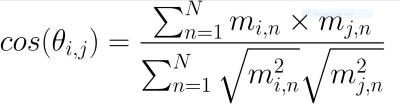
attr(vals_t, "dimnames") <- NULLCosine similarity is a common method used in recommender systems to identify similar entities (books, movies, etc.) on the basis of a vector of data features. In the previous block of code, we created and (N x M) matrix where N is the number of features in the data set and M is the number of counties. Cosine similarity works by calculating the angle (θᵢ,ⱼ) from the edges formed between the column vector of the focal county (mᵢ) and a comparison county (mⱼ) in n-dimensional space. The cosine of two vectors that share many properties will have an angle close to 0 and therefore a cosine value near 1. Conversely, dissimilar counties will have lower scores because the angle of their edge will be larger. The formula for calculating cosine similarity is as follows:
余弦相似度是推荐系统中基于数据特征向量识别相似实体(书籍,电影等)的常用方法。 在上一个代码块中,我们创建了(N x M)矩阵,其中N是数据集中的要素数量,M是县数量。 余弦相似度是通过计算n维空间中焦点县(mᵢ)和比较县(mⱼ)的列向量之间形成的边缘的角度(θᵢ,ⱼ)来进行的。 具有许多特性的两个向量的余弦将具有接近0的角度,因此余弦值接近1。相反,相异的县的得分较低,因为它们的边缘角度会更大。 余弦相似度的计算公式如下:
The code for this calculation is given below along with an example for Cook County, Illinois, which includes the city of Chicago.
下面给出了此计算的代码,并提供了一个伊利诺伊州库克县的示例,其中包括芝加哥市。
cosine_similarity <- function(x, focal_index, measure = "angle") {
  assertthat::assert_that(measure %in% c("angle", "distance"),
                          length(measure) == 1)
  cos_prox = rep(NA, ncol(x))
  for (i in 1:ncol(x)) {
    if (focal_index != i) {
      A = x[, focal_index] %>%
        as.matrix(ncol = 1)
      A_norm = (A * A)  %>% sum() %>% sqrt()
      B = x[, i] %>%
        as.matrix(ncol = 1)
      B_norm = (B * B)  %>% sum() %>% sqrt()
      dot_AB = sum(A * B)
      cos_prox[i] = dot_AB / (A_norm * B_norm)
    }
  }
  if (measure=="angle")
    return(cos_prox)
  else
    cos_distance = acos(cos_prox) / pi
    return(cos_distance)
}
#Measure cosine distance among counties, relative to focal county
focal_location <- "cook,_illinois"
focal_index <-
  which(d$name == focal_location) #index of focal location
d$cosine_sim <- cosine_similarity(vals_t, focal_index, measure = "angle")#Top 10 Recommendations
d[order(d$cosine_sim,decreasing = TRUE),c("name","cosine_sim")]## Simple feature collection with 3076 features and 2 fields
## geometry type:  MULTIPOLYGON
## dimension:      XY
## bbox:           xmin: -124.6813 ymin: 25.12993 xmax: -67.00742 ymax: 49.38323
## CRS:            +proj=longlat +ellps=WGS84
## First 10 features:
##                            name cosine_sim                       geometry
## 1194     suffolk,_massachusetts  0.9367209 MULTIPOLYGON (((-71.17855 4...
## 710             marion,_indiana  0.9346767 MULTIPOLYGON (((-86.31609 3...
## 1816            kings,_new_york  0.9300806 MULTIPOLYGON (((-73.86572 4...
## 3018       milwaukee,_wisconsin  0.9080851 MULTIPOLYGON (((-88.06934 4...
## 1740       atlantic,_new_jersey  0.9072181 MULTIPOLYGON (((-74.98299 3...
## 1852      westchester,_new_york  0.8982588 MULTIPOLYGON (((-73.80843 4...
## 279       hartford,_connecticut  0.8946008 MULTIPOLYGON (((-72.74845 4...
## 2259 philadelphia,_pennsylvania  0.8916324 MULTIPOLYGON (((-74.97153 4...
## 217          arapahoe,_colorado  0.8858975 MULTIPOLYGON (((-104.6565 3...
## 2253       monroe,_pennsylvania  0.8852190 MULTIPOLYGON (((-74.98299 4...
The Top 10 recommendations for Cook County residents are presented here. Most similar to Cook County are Suffolk County, MA, a suburb of New York City, and Marion County, IN, which contains the city of Indianapolis.
这里介绍了对库克县居民的十大建议。 与库克县最相似的是位于纽约市郊区的马萨诸塞州萨福克县和包含印第安纳波利斯市的印第安纳州马里恩县。
结论 (Conclusion)
This was a quick overview of the data and methods that went into Niche: An Interface for Exploring Relocation Options. If you would like to give a try, visit the most up-to-date version on my Shinyapps page (https://ericvc.shinyapps.io/Niche/) or clone the GitHub directory and run the app from your computer with RStudio. Note, the app.R file contains code for initializing a Python virtual environment (using the reticulate package), which Niche requires in order to function completely. This code causes issues when executed on my local system. Commenting out the code fixes the issue, but are otherwise required when running the hosted version of the program. Some features will not be available without the ability to execute Python code.
这是Niche:探索重定位选项的接口所使用的数据和方法的快速概述。 如果您想尝试一下,请访问我的Shinyapps页面上的最新版本(https://ericvc.shinyapps.io/Niche/)或克隆GitHub目录,然后使用RStudio从计算机上运行该应用程序。 请注意, app.R文件包含用于初始化Python虚拟环境(使用reticulate软件包)的代码,Niche需要此代码才能完全运行。 在我的本地系统上执行时,此代码会导致问题。 注释掉该代码可解决此问题,但在运行程序的托管版本时则需要这样做。 如果没有执行Python代码的功能,某些功能将不可用。
The purpose of Niche is to help guide users’ relocation research by translating their personal preferences and past experiences into a data-centric model in order to make recommendations. Some future plans for this tool include adding historical data that would allow users to find locations in the present that are similar to a location and time from the recent past (e.g., within the last 20 years or so).
Niche的目的是通过将用户的个人偏好和过去的经验转化为以数据为中心的模型来提出建议,从而帮助指导用户进行搬迁研究。 该工具的一些未来计划包括添加历史数据,该历史数据将允许用户查找与最近的过去(例如,最近20年左右)的地点和时间相似的地点。
翻译自: https://medium.com/@ericvc2/niche-an-interface-for-exploring-your-moving-options-858a0baa29b2
ajax不利于seo
本文来自互联网用户投稿,该文观点仅代表作者本人,不代表本站立场。本站仅提供信息存储空间服务,不拥有所有权,不承担相关法律责任。如若转载,请注明出处:http://www.luyixian.cn/news_show_707652.aspx
如若内容造成侵权/违法违规/事实不符,请联系dt猫网进行投诉反馈email:809451989@qq.com,一经查实,立即删除!相关文章

如何优化网站加载时间
鲜为人知的6个黑科技网站_6种鲜为人知的熊猫绘图工具


新版 Android 已支持 FIDO2 标准,免密登录应用或网站

【百度】大型网站的HTTPS实践(一)——HTTPS协议和原理

COOKIE伪造登录网站后台

phpstudy如何安装景安ssl证书 window下apache服务器网站https访问

【计算机网络】手动配置hosts文件解决使用GitHub和Coursera网站加载慢/卡的问题
小白创建网站的曲折之路
html在线编辑器 asp.net,ASP.NET网站使用Kindeditor富文本编辑器配置步骤
![大型网站服务器 pdf,大型网站服务器容量规划[PDF][145.25MB]](https://img-blog.csdnimg.cn/img_convert/d69c7a6a67a3f04be90eedc900601efa.png)
大型网站服务器 pdf,大型网站服务器容量规划[PDF][145.25MB]

怎么暂时关闭网站php,WordPress怎么临时关闭网站进行维护

17joys网站后台功能设计-阶段1

拉拢中小网站 淘宝百度暗战升级...

10款精选的用于构建良好易用性网站的jQuery插件

A4Desk 网站破解

IIS7 MVC网站生成、发布
