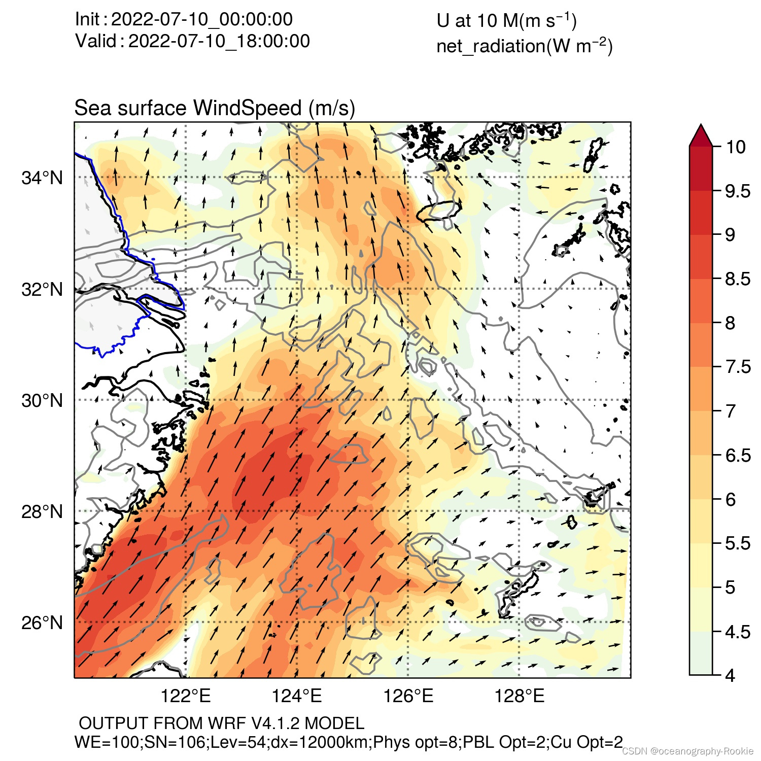
使用python自动化绘制WRF模式输出的风场以及辐射

本脚本主要用来自动化处理WRF模式数据，可以根据自己指定的时间范围以及时间步长绘制相应的数据

1 导入库

import cmaps
import numpy as np
import glob
from netCDF4 import Dataset
import matplotlib.pyplot as plt
from matplotlib.cm import get_cmap
import cartopy.crs as crs
from cartopy.feature import NaturalEarthFeature
from cartopy.mpl.ticker import LongitudeFormatter, LatitudeFormatter
from wrf import (to_np, getvar, smooth2d, get_cartopy, cartopy_xlim,cartopy_ylim, latlon_coords,extract_global_attrs)
import proplot as pplt
import pandas as pd
import datetime
import os

2 选择数据范围

需要自己手动选择：初始时间、结束时间、时间步长

输入格式为：年-月-日-时、年-月-日-时、时
2022071000
2022071012
03

date = input()
frst = input()
step = input()path = r'G:/'+ date #只能是已经存在的文件目录且有数据才可以进行读取start = datetime.datetime.strptime(date,'%Y%m%d%H').strftime("%Y-%m-%d_%H_%M_%S")end = (datetime.datetime.strptime(date,'%Y%m%d%H')+datetime.timedelta(hours=int(frst))).strftime("%Y-%m-%d_%H_%M_%S")intp = (datetime.datetime.strptime(date,'%Y%m%d%H')+datetime.timedelta(hours=int(step))).strftime("%Y-%m-%d_%H_%M_%S")fstart = path+'/*'+start
fintp  = path+'/*'+intp
fend   = path+'/*'+endfile = path+'/*'filestart = glob.glob(fstart)
fileintp = glob.glob(fintp)
fileend = glob.glob(fend)filelist  = glob.glob(file)filelist.sort()   rstart = np.array(np.where(np.array(filelist)==filestart))[0][0]
rintp = np.array(np.where(np.array(filelist)==fileintp))[0][0]
rend   = np.array(np.where(np.array(filelist)==fileend))[0][0]

3定义读取数据函数以及绘图函数

定义函数读取风速资料U、V，以及辐射（辐射包括三部分）

将读取的资料进行绘图，并将绘图后的结果自动保存到指定路径下，方面后续绘制动图

def plot(i):ncfile = Dataset(i)#get u10 v10u10 = getvar(ncfile,'U10')v10 = getvar(ncfile,'V10')w10 = np.sqrt(u10*u10+v10*v10)#get net_radswdown = getvar(ncfile,'SWDOWN')glw    = getvar(ncfile,'GLW')olr    = getvar(ncfile,'OLR')rad    = swdown+glw+olrWE = extract_global_attrs(ncfile,'WEST-EAST_GRID_DIMENSION')['WEST-EAST_GRID_DIMENSION']SN = extract_global_attrs(ncfile,'SOUTH-NORTH_GRID_DIMENSION')['SOUTH-NORTH_GRID_DIMENSION']lev= extract_global_attrs(ncfile,'BOTTOM-TOP_GRID_DIMENSION')['BOTTOM-TOP_GRID_DIMENSION']t =u10.Time# time = pd.to_datetime((t)).strftime('%Y-%m-%d-%H')# Get the latitude and longitude pointslats, lons = latlon_coords(u10)# Create a figuref = pplt.figure(figsize=(5,5))ax = f.subplot(111, proj='lcyl')m=ax.contourf(to_np(lons), to_np(lats), to_np(w10),cmap=cmaps.MPL_RdYlBu_r,levels=np.arange(4,10.5,0.5),extend='both')ax.contour(to_np(lons), to_np(lats), to_np(rad),levels=8,linewidth=0.9,color='grey',# cmap=cmaps.MPL_RdYlBu_r,)step=4ax.quiver(to_np(lons)[::step,::step],to_np(lats)[::step,::step],to_np(u10)[::step,::step],to_np(v10)[::step,::step],)ax.format(ltitle='Sea surface WindSpeed (m/s)',coast=True,labels=True,lonlim=(120, 130),latlines=2,lonlines=2,latlim=(25, 35),)props = dict(boxstyle='round', facecolor='wheat', alpha=0.5)bbox_props = dict(boxstyle="round", fc="w", ec="0.5", alpha=1)textstr = '\n'.join((r'$  Init:$'+ ncfile.START_DATE,r'$Valid:$' + i[-19:],# r'$\sigma=%.2f$' % (2, ))))ax.text(0.0, 1.2, textstr, transform=ax.transAxes, fontsize=9,verticalalignment='top', )ax.text(0.65, 1.2, 'U at 10 M(m s$^{-1}$)'+'\n'+'net_radiation(W m$^{-2}$)', transform=ax.transAxes, fontsize=9,verticalalignment='top', )ax.text(0.00, -0.07, ncfile.TITLE+'\n'+r'WE='+str(WE)+';SN='+str(SN)+';Lev='+str(lev)+';dx='+str(int(ncfile.DX))+'km;'+'Phys opt='+str(ncfile.MP_PHYSICS)+';PBL Opt='+str(ncfile.BL_PBL_PHYSICS)+';Cu Opt='+str(ncfile.CU_PHYSICS),fontsize=8,horizontalalignment='left',verticalalignment='top',transform=ax.transAxes,)f.colorbar(m, loc='r',label='',length=0.75,width=0.15)plt.show()savepath = r'J:/'+ dateif not os.path.exists(savepath):os.makedirs(savepath)f.savefig(savepath+'\\uv10'+i[-19:]+'.jpg')return

4 定义代码运行函数。

def plot_uv(fn):for i  in fn:plot(i)print('finish'+i)returnif __name__ == "__main__":plot_uv(fn)print('uvplot is finish')

5 个例测试

方面数据测试，取削封装函数运行。

path = r'G:\2022071000/*'file = glob.glob(path)file.sort()ncfile = Dataset(file[0])#get u10 v10
u10 = getvar(ncfile,'U10')
v10 = getvar(ncfile,'V10')
w10 = np.sqrt(u10*u10+v10*v10)
#get net_rad
swdown = getvar(ncfile,'SWDOWN')
glw    = getvar(ncfile,'GLW')
olr    = getvar(ncfile,'OLR')rad    = swdown+glw+olrWE = extract_global_attrs(ncfile,'WEST-EAST_GRID_DIMENSION')['WEST-EAST_GRID_DIMENSION']
SN = extract_global_attrs(ncfile,'SOUTH-NORTH_GRID_DIMENSION')['SOUTH-NORTH_GRID_DIMENSION']
lev= extract_global_attrs(ncfile,'BOTTOM-TOP_GRID_DIMENSION')['BOTTOM-TOP_GRID_DIMENSION']t =datetime.datetime.strptime(u10.Time.values,'%Y%m%d%H').strftime("%Y-%m-%d_%H_%M_%S")
# time = pd.to_datetime((t)).strftime('%Y-%m-%d-%H')# Get the latitude and longitude points
lats, lons = latlon_coords(u10)# Create a figure
f = pplt.figure(figsize=(5,5))
ax = f.subplot(111, proj='lcyl')m=ax.contourf(to_np(lons), to_np(lats), to_np(w10),cmap=cmaps.MPL_RdYlBu_r,)
ax.contour(to_np(lons), to_np(lats), to_np(rad),levels=8,linewidth=0.9,color='grey',# cmap=cmaps.MPL_RdYlBu_r,)
step=4
ax.quiver(to_np(lons)[::step,::step],to_np(lats)[::step,::step],to_np(u10)[::step,::step],to_np(v10)[::step,::step],)ax.format(ltitle='Sea surface WindSpeed (m/s)',coast=True,labels=True,lonlim=(120, 130),latlines=2,lonlines=2,latlim=(25, 35),)props = dict(boxstyle='round', facecolor='wheat', alpha=0.5)bbox_props = dict(boxstyle="round", fc="w", ec="0.5", alpha=1)textstr = '\n'.join((r'$  Init:$'+ ncfile.START_DATE,r'$Valid:$' + file[],# r'$\sigma=%.2f$' % (2, ))))
ax.text(0.0, 1.2, textstr, transform=ax.transAxes, fontsize=9,verticalalignment='top', )ax.text(0.65, 1.2, 'U at 10 M(m s$^{-1}$)'+'\n'+'net_radiation(W m$^{-2}$)', transform=ax.transAxes, fontsize=9,verticalalignment='top', )ax.text(0.00, -0.07, ncfile.TITLE+'\n'+r'WE='+str(WE)+';SN='+str(SN)+';Lev='+str(lev)+';dx='+str(int(ncfile.DX))+'km;'+'Phys opt='+str(ncfile.MP_PHYSICS)+';PBL Opt='+str(ncfile.BL_PBL_PHYSICS)+';Cu Opt='+str(ncfile.CU_PHYSICS),fontsize=8,horizontalalignment='left',verticalalignment='top',transform=ax.transAxes,)f.colorbar(m, loc='r',label='',length=0.75,width=0.15)
plt.show()
# f.savefig('J:\\20220710\\'+i[35:]+'.png')# for i in file:#     plot_p(i)#     print('finish'+i)# print(i)


# -*- coding: utf-8 -*-
"""
Created on %(date)s@author: %(jixianpu)sEmail : 211311040008@hhu.edu.cnintroduction : keep learning althongh walk slowly
"""
"""
introduction :绘制近地面的风场和辐射
"""
import cmaps
import numpy as np
import glob
from netCDF4 import Dataset
import matplotlib.pyplot as plt
from matplotlib.cm import get_cmap
import cartopy.crs as crs
from cartopy.feature import NaturalEarthFeature
from cartopy.mpl.ticker import LongitudeFormatter, LatitudeFormatter
from wrf import (to_np, getvar, smooth2d, get_cartopy, cartopy_xlim,cartopy_ylim, latlon_coords,extract_global_attrs)
import proplot as pplt
import pandas as pd
import datetime
import osdate = input()
frst = input()
step = input()path = r'G:/'+ date #只能是已经存在的文件目录且有数据才可以进行读取start = datetime.datetime.strptime(date,'%Y%m%d%H').strftime("%Y-%m-%d_%H_%M_%S")end = (datetime.datetime.strptime(date,'%Y%m%d%H')+datetime.timedelta(hours=int(frst))).strftime("%Y-%m-%d_%H_%M_%S")intp = (datetime.datetime.strptime(date,'%Y%m%d%H')+datetime.timedelta(hours=int(step))).strftime("%Y-%m-%d_%H_%M_%S")fstart = path+'/*'+start
fintp  = path+'/*'+intp
fend   = path+'/*'+endfile = path+'/*'filestart = glob.glob(fstart)
fileintp = glob.glob(fintp)
fileend = glob.glob(fend)filelist  = glob.glob(file)filelist.sort()   rstart = np.array(np.where(np.array(filelist)==filestart))[0][0]
rintp = np.array(np.where(np.array(filelist)==fileintp))[0][0]
rend   = np.array(np.where(np.array(filelist)==fileend))[0][0]fn = filelist[rstart:rend:rintp]
# fn = filelist[rstart:rend:rintp]def plot(i):ncfile = Dataset(i)#get u10 v10u10 = getvar(ncfile,'U10')v10 = getvar(ncfile,'V10')w10 = np.sqrt(u10*u10+v10*v10)#get net_radswdown = getvar(ncfile,'SWDOWN')glw    = getvar(ncfile,'GLW')olr    = getvar(ncfile,'OLR')rad    = swdown+glw+olrWE = extract_global_attrs(ncfile,'WEST-EAST_GRID_DIMENSION')['WEST-EAST_GRID_DIMENSION']SN = extract_global_attrs(ncfile,'SOUTH-NORTH_GRID_DIMENSION')['SOUTH-NORTH_GRID_DIMENSION']lev= extract_global_attrs(ncfile,'BOTTOM-TOP_GRID_DIMENSION')['BOTTOM-TOP_GRID_DIMENSION']t =u10.Time# time = pd.to_datetime((t)).strftime('%Y-%m-%d-%H')# Get the latitude and longitude pointslats, lons = latlon_coords(u10)# Create a figuref = pplt.figure(figsize=(5,5))ax = f.subplot(111, proj='lcyl')m=ax.contourf(to_np(lons), to_np(lats), to_np(w10),cmap=cmaps.MPL_RdYlBu_r,levels=np.arange(4,10.5,0.5),extend='both')ax.contour(to_np(lons), to_np(lats), to_np(rad),levels=8,linewidth=0.9,color='grey',# cmap=cmaps.MPL_RdYlBu_r,)step=4ax.quiver(to_np(lons)[::step,::step],to_np(lats)[::step,::step],to_np(u10)[::step,::step],to_np(v10)[::step,::step],)ax.format(ltitle='Sea surface WindSpeed (m/s)',coast=True,labels=True,lonlim=(120, 130),latlines=2,lonlines=2,latlim=(25, 35),)props = dict(boxstyle='round', facecolor='wheat', alpha=0.5)bbox_props = dict(boxstyle="round", fc="w", ec="0.5", alpha=1)textstr = '\n'.join((r'$  Init:$'+ ncfile.START_DATE,r'$Valid:$' + i[-19:],# r'$\sigma=%.2f$' % (2, ))))ax.text(0.0, 1.2, textstr, transform=ax.transAxes, fontsize=9,verticalalignment='top', )ax.text(0.65, 1.2, 'U at 10 M(m s$^{-1}$)'+'\n'+'net_radiation(W m$^{-2}$)', transform=ax.transAxes, fontsize=9,verticalalignment='top', )ax.text(0.00, -0.07, ncfile.TITLE+'\n'+r'WE='+str(WE)+';SN='+str(SN)+';Lev='+str(lev)+';dx='+str(int(ncfile.DX))+'km;'+'Phys opt='+str(ncfile.MP_PHYSICS)+';PBL Opt='+str(ncfile.BL_PBL_PHYSICS)+';Cu Opt='+str(ncfile.CU_PHYSICS),fontsize=8,horizontalalignment='left',verticalalignment='top',transform=ax.transAxes,)f.colorbar(m, loc='r',label='',length=0.75,width=0.15)plt.show()savepath = r'J:/'+ dateif not os.path.exists(savepath):os.makedirs(savepath)f.savefig(savepath+'\\uv10'+i[-19:]+'.jpg')returndef plot_uv(fn):for i  in fn:plot(i)print('finish'+i)returnif __name__ == "__main__":plot_uv(fn)print('uvplot is finish')