算例路径: olaFlow\tutorials\baseWaveFlume
算例描述: 一个基础的二维波浪水槽
算例快照:


文件结构:
├── 0.org
│   ├── U
│   ├── alpha.water
│   ├── alpha.water.org
│   └── p_rgh
├── cleanCase
├── constant
│   ├── dynamicMeshDict
│   ├── g
│   ├── transportProperties
│   ├── turbulenceProperties
│   └── waveDict   --> 设置波浪要素
├── runCase
└── system├── blockMeshDict├── controlDict├── decomposeParDict├── fvSchemes├── fvSolution└── setFieldsDict  --> 设置水深
算例文件解析:
【0.org\U】
dimensions      [0 1 -1 0 0 0 0];  // 量纲 m/s
internalField   uniform (0 0 0);   // 内部速度场 均一场 0 0 0
boundaryField   //边界场
{inlet      // 造波边界{type            waveVelocity; // 波浪速度waveDictName    waveDict;     // 读取constant\waveDict中的波浪要素value           uniform (0 0 0);  //初值为 0 0 0}outlet    // 消波边界{type            waveAbsorption2DVelocity;  // 使用了二维消波理论,olaFlow采用主动消波法value           uniform (0 0 0);}bottom   // 底部边界为固壁边界,边界上速度为零{type            fixedValue;   value           uniform (0 0 0);}atmosphere // 大气边界,允许空气流出和流入{type            pressureInletOutletVelocity;value           uniform (0 0 0);}frontAndBack // 前后面,empty指示模型为二维模型{type            empty;}
}
【0.org\p_rgh】
// p_rgh = p - rgh,实际压力减去静水压力
dimensions      [1 -1 -2 0 0 0 0];  // M(1) L(-1) T(-2)
internalField   uniform 0;
boundaryField
{frontAndBack{type            empty;}outlet{type            fixedFluxPressure; //将压力梯度设置为0,边界上的通量由速度边界条件指定value           uniform 0;}inlet {type            fixedFluxPressure;value           uniform 0;}bottom{type            fixedFluxPressure;value           uniform 0;}atmosphere {type            totalPressure; //总压条件:流出 p = p0; 流入 p = p0 - 0.5|U|^2U               U;phi             phi;rho             rho;psi             none;gamma           1;p0              uniform 0;value           uniform 0;}
}
【0.org\alpha.water.org】
// 设置流体体积分数
dimensions      [0 0 0 0 0 0 0];
internalField   uniform 0;
boundaryField
{inlet{type            waveAlpha;  // 根据波浪条件设置waveDictName    waveDict;value           uniform 0;}frontAndBack{type            empty;}outlet{type            zeroGradient; // 零梯度}bottom{type            zeroGradient;}atmosphere{type            inletOutlet; // 当流体流出时,α的梯度为0;如果流入,α为0,100%的空气流入inletValue      uniform 0;value           uniform 0;}
}
【constant\dynamicMeshDict】
dynamicFvMesh staticFvMesh;
【constant\g】
dimensions      [0 1 -2 0 0 0 0];
value           ( 0 0 -9.81 );
【constant\transportProperties】
phases (water air);water
{transportModel  Newtonian;nu              [0 2 -1 0 0 0 0] 1e-06;  // 流体运动粘度rho             [1 -3 0 0 0 0 0] 1000;   // 流体密度
}air
{transportModel  Newtonian;nu              [0 2 -1 0 0 0 0] 1.48e-05;rho             [1 -3 0 0 0 0 0] 1;
}sigma           [1 0 -2 0 0 0 0] 0.07;     // 水和空气之间的表面张力参数
【constant\turbulenceProperties】
simulationType laminar; // 设置为层流模型
【constant\waveDict】
waveType        regular;    // 规则波
waveTheory      cnoidal;    // 椭圆余弦波
genAbs          1;          // 考虑造波边界的消波性能  1/0
absDir          0.0;        // 造波边界的消波方向
nPaddles        1;          // 主动消波的Paddles数量设置
waveHeight      0.10;       // 波高
wavePeriod      3;          // 波周期
waveDir         0.0;        // 波向
wavePhase       1.57079633; // 初始相位
// Change both entries to true to re-read this dictionary upon restart.
rereadAlpha     false;
rereadU         false;
【system\blockMeshDict】
scale 1;
vertices
((0.0     -0.02   0.0)(10.0    -0.02   0.0)(10.0    -0.02   0.7)(0.0     -0.02   0.7)(0.0     0.0     0.0)(10.0    0.0     0.0)(10.0    0.0     0.7)(0.0     0.0     0.7)
);
blocks
(hex (0 1 5 4 3 2 6 7)   (500 1 70) simpleGrading (1 1 1)
);
edges
(
);
patches
(patch inlet  // 造波边界((0 4 7 3))patch outlet  // 消波边界 ((1 5 6 2))wall bottom   // 水槽底部边界((0 1 5 4))patch atmosphere  // 大气边界((3 2 6 7))empty frontAndBack // 水槽侧面边界((0 1 2 3)(4 5 6 7))
);
mergePatchPairs
(
);
【system\controlDict】
application     olaFlow;      // olaFlow求解器
startFrom       latestTime;
startTime       0;
stopAt          endTime;
endTime         60;
deltaT          0.001;       // 计算时间步
writeControl    adjustableRunTime;
writeInterval   0.05;        // 写出时间步
purgeWrite      0;
writeFormat     ascii;
writePrecision  6;
compression     off;         // 是否压缩格式写出,可节约硬盘空间, on/off
timeFormat      general;
timePrecision   6;
runTimeModifiable yes;
adjustTimeStep  yes;         // 采用自适应时间步,可能会加速计算,也可能造成时间步极小
maxCo           0.5;         // CFL条件的Courant数, 一般<1, 设置一个小值会使计算结果更精确,但也减小了时间步长,增加了计算成本
maxAlphaCo	    0.5;         // 两相交界面上的最大Courant数
maxDeltaT       0.025;
【system\decomposeParDict】
numberOfSubdomains 2;        // 并行区域分解数目
method          scotch;      // 区域分解方法
...
【system\fvSchemes】
// 指定控制方程中各项的有限体积法的离散格式
ddtSchemes  // 指定时间离散格式
{default         Euler;  // Euler法,一阶精度,条件稳定
} gradSchemes  // 梯度项离散格式
{default         Gauss linear; // 高斯定理,将网格中心的量插值到网格面上
}// olaFlow 的算例中给出了几乎所有可能出现的项,具体算例可能不会包含全部项
divSchemes  // 对流项与散度项的离散格式, 将网格中心的量插值到网格面上,因此实际上选用的是interpolationSchemes
{div(rhoPhi,U)  Gauss limitedLinearV 1;  // Guass limitedLinear(一种TVD格式,使同时满足精度和有界) V类(采用限制器时考虑了流动方向)div(U)  Gauss linear; // 二阶精度,无界div((rhoPhi|interpolate(porosity)),U)  Gauss limitedLinearV 1;div(rhoPhiPor,UPor)  Gauss limitedLinearV 1;div(rhoPhi,UPor)  Gauss limitedLinearV 1;div(rhoPhiPor,U)   Gauss limitedLinearV 1; div(phi,alpha)  Gauss vanLeer; // Gauss vanLeer(一种TVD格式,使同时满足精度和有界)div(phirb,alpha) Gauss interfaceCompression; // 界面压缩格式,基于一般限制格式div((muEff*dev(T(grad(U))))) Gauss linear;div(phi,k)      Gauss upwind; // 一阶迎风格式,有界div(phi,epsilon) Gauss upwind;div((phi|interpolate(porosity)),k)      Gauss upwind;div((phi|interpolate(porosity)),epsilon) Gauss upwind;div(phi,omega) Gauss upwind;div((phi|interpolate(porosity)),omega) Gauss upwind;
}laplacianSchemes  // 拉普拉斯项离散格式
{default         Gauss linear corrected; // Guass线性插值,corrected(显式的非正交网格修正)
}interpolationSchemes
{default         linear;  // 线性插值格式
}snGradSchemes  // 面法向梯度格式
{default         corrected;
}fluxRequired  //
{default         no;p_rgh;pcorr;alpha.water;
}
【system\fvSolution】
// 指定方程组矩阵求解器、残差以及其他算法控制
solvers
{"alpha.water.*"{nAlphaCorr      1;  //nAlphaSubCycles 2;alphaOuterCorrectors yes;cAlpha          1;MULESCorr       no;nLimiterIter    3;solver          smoothSolver;    // 求解器:光顺求解器。对称和非对称矩阵均适用smoother        symGaussSeidel;  // 光顺器:对称Gauss-Seidel方法tolerance       1e-8;            // 标准化残差relTol          0;               // 相对残差,表征残差的递减量}"pcorr.*"  // 压强校正量{solver          PCG;            // 求解器:预处理共轭梯度法。仅适用于对称矩阵    preconditioner  DIC;            // 预处理器:基于对角的不完全Cholesky预处理器tolerance       1e-5;relTol          0;}p_rgh{solver          PCG;preconditioner  DIC;tolerance       1e-07;relTol          0.05;}p_rghFinal  // 在求解p_rgh时可设置较大的残差,在最后一步设置严格的误差{$p_rgh;relTol          0;}U{solver          smoothSolver; smoother        symGaussSeidel;tolerance       1e-06;relTol          0;}
}// 离散方程组的分离式解法
PIMPLE   // SIMPLE 与 PISO 算法的耦合
{momentumPredictor   no;nOuterCorrectors    1;  // 值不大于1时,算法变为纯PISO算法;若大于1,为非定常SIMPLE算法nCorrectors         3;nNonOrthogonalCorrectors 0;
}relaxationFactors // 松弛方法,为降低数值波动
{fields        // 表示需要使用松弛方法(显式)的变量{}equations     // 表示需要使用松弛方法(隐式)的方程{".*" 1;}
}
【system\setFieldsDict】
defaultFieldValues
(volScalarFieldValue alpha.water 0   // 初始化流体体积分数
);
regions
(boxToCell{box (-10 -1 -1) (30 1 0.4);fieldValues(volScalarFieldValue alpha.water 1  // 将box范围内的流体设置为a = 1的相,即水深);}
);