1. 使用python和numpy实现一个线性回归

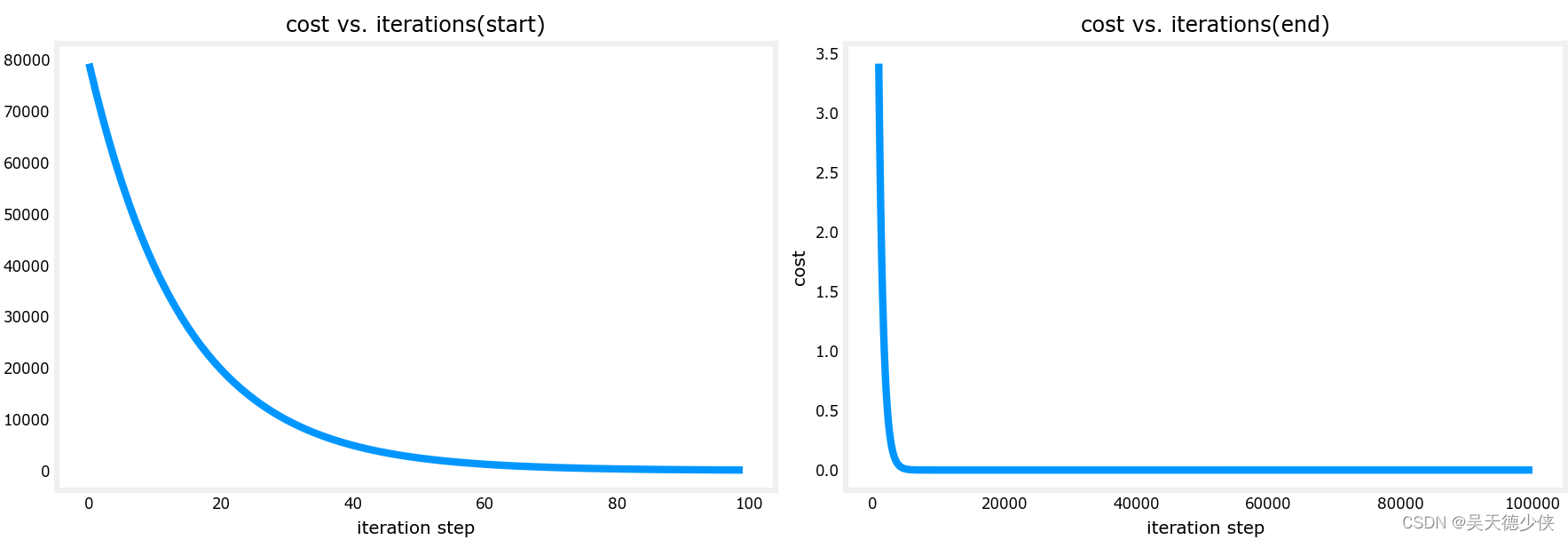
要求使用梯度下降法，可视化$loss$随着迭代次数的变化曲线

2. 说明

2.1 拟合函数

$f_{w,b}(x^{(i)})=w{x}^{(i)}+b$

2.2 均方误差损失函数

$J(w,b)=\frac{1}{2m}\sum _{i=0}^{m-1}(f_{w,b}(x^{(i)})-y^{(i)}{)}^2$
重复进行：

• $w=w-\alpha \frac{\partial J(w,b)}{\partial w}$
• $b=b-\alpha \frac{\partial J(w,b)}{\partial b}$

2.3 需要实现3个方法

• 计算梯度
• 计算损失
• 梯度下降

3. 代码

3.1 gradient_descent_sln.py

from distutils.command.bdist_wininst import bdist_wininst
import numpy as np
import math
import copy
import matplotlib.pyplot as pltplt.style.use("deeplearning.mplstyle")
from lab_utils_uni import (plt_house_x,plt_contour_wgrad,
plt_divergence,plt_gradients)def compute_cost(x,y,w,b):"""function to calculate the cost"""m = x.shape[0]cost = 0for i in range(m):f_wb = w*x[i]+bcost = cost + (f_wb - y[i])**2total_cost = 1/(2*m)*cost # 根据公式return total_costdef compute_gradient(x,y,w,b):"""compute the gradient for linear regression\nx: (ndarray,(m,)): data,m examples\ny: (ndarray,(m,)): target values\nw,b (scalar)     : model parameters\nreturn:\ndj_dw (scalar)  : the gradient of the cost w.r.t the parameter w\ndj_db (scalar)  : the gradient of the cost w.r.t the parameter b\n"""# number of training examplesm = x.shape[0]dj_dw = 0dj_db = 0for i in range(m):f_wb = w * x[i] + bdj_dw_i = (f_wb-y[i])*x[i]dj_db_i = (f_wb-y[i])dj_db +=dj_db_idj_dw +=dj_dw_idj_dw = dj_dw/mdj_db = dj_db/mreturn dj_dw,dj_dbdef gradient_descent(x,y,w_in,b_in,alpha,num_iters,cost_function,gradient_function):w = copy.deepcopy(w_in)J_history = [] # 损失值p_history = [] # 参数值b = b_inw = w_infor i in range(num_iters):dj_dw,dj_db = gradient_function(x,y,w,b)# updateb = b - alpha * dj_dbw = w - alpha * dj_dw# 保存历史损失值if i<1e5:J_history.append(cost_function(x,y,w,b))p_history.append([w,b])# 每10个迭代输出一次历史信息if i%math.ceil(num_iters/10)==0:print(f'Iteration {i:4}: Cost {J_history[-1]:.2e} ',f'dj_dw: {dj_dw:.3e}, dj_db: {dj_db:.3e} ',f'w: {w:.3e}, b:{b:.5e}')return w,b,J_history,p_history        if __name__ == '__main__':print("program start".center(60,'='))# load datasetx_train = np.array([1.0,2.0])y_train = np.array([300,500])# 显示损失函数plt_gradients(x_train,y_train,compute_cost,compute_gradient)plt.show()# initialize parametersw_init = 0b_init = 0# hyper parametersiterations = int(1e5)tmp_alpha = 1e-2# run itw_final,b_final,J_hist,p_hist = gradient_descent(x_train,y_train,w_init,b_init,tmp_alpha,iterations,compute_cost,compute_gradient)print(f'(w,b) found by gradient descent: ({w_final:8.4f}, {b_final:8.4f})')# plot cost vs iterationsfig,(ax1,ax2) = plt.subplots(1,2,constrained_layout=True,figsize=(12,4))ax1.plot(J_hist[:100])ax2.plot(1000+np.arange(len(J_hist[1000:])),J_hist[1000:])ax1.set_title("cost vs. iterations(start)")ax2.set_title("cost vs. iterations(end)")ax1.set_ylabel("cost")ax2.set_ylabel("cost")ax1.set_xlabel("iteration step")ax2.set_xlabel("iteration step")plt.show()

3.2 结果

=======================program start========================Iteration    0: Cost 7.93e+04  dj_dw: -6.500e+02, dj_db: -4.000e+02  w: 6.500e+00, b:4.00000e+00
Iteration 10000: Cost 6.74e-06  dj_dw: -5.215e-04, dj_db: 8.439e-04  w: 2.000e+02, b:1.00012e+02
Iteration 20000: Cost 3.09e-12  dj_dw: -3.532e-07, dj_db: 5.714e-07  w: 2.000e+02, b:1.00000e+02
Iteration 30000: Cost 1.42e-18  dj_dw: -2.393e-10, dj_db: 3.869e-10  w: 2.000e+02, b:1.00000e+02
Iteration 40000: Cost 1.26e-23  dj_dw: -1.421e-12, dj_db: 7.105e-13  w: 2.000e+02, b:1.00000e+02
Iteration 50000: Cost 1.26e-23  dj_dw: -1.421e-12, dj_db: 7.105e-13  w: 2.000e+02, b:1.00000e+02
Iteration 60000: Cost 1.26e-23  dj_dw: -1.421e-12, dj_db: 7.105e-13  w: 2.000e+02, b:1.00000e+02
Iteration 70000: Cost 1.26e-23  dj_dw: -1.421e-12, dj_db: 7.105e-13  w: 2.000e+02, b:1.00000e+02
Iteration 80000: Cost 1.26e-23  dj_dw: -1.421e-12, dj_db: 7.105e-13  w: 2.000e+02, b:1.00000e+02
Iteration 90000: Cost 1.26e-23  dj_dw: -1.421e-12, dj_db: 7.105e-13  w: 2.000e+02, b:1.00000e+02
(w,b) found by gradient descent: (200.0000, 100.0000)