G:\r\tcga_example-master\scripts

library(survival)
library(survminer)## 批量生存分析 使用 coxph 回归方法
# http://www.sthda.com/english/wiki/cox-proportional-hazards-model
colnames(phe)
head(phe)     #event中1 表示存活（终点事件）
#https://rpubs.com/kaz_yos/survival-auc
mySurv=with(phe,Surv(time, event))    # ## Create a survival vector
head(mySurv)      #surv的结果只是一列一连串的生存时间汇总。所以一般会提倡用phe$mysurv这种方式把结果整合到原始数据框中便于之后的分析
#生存曲线与结果汇总

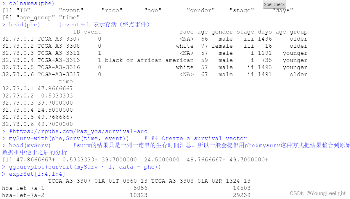
ggsurvplot(survfit(mySurv ~ 1, data = phe))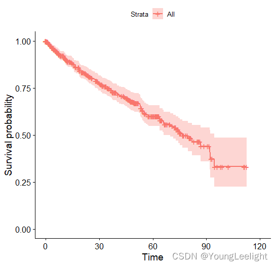

ggsurvplot(survfit(mySurv ~ age_group, data = phe),  label.curves = list(method = "arrow", cex = 1.2))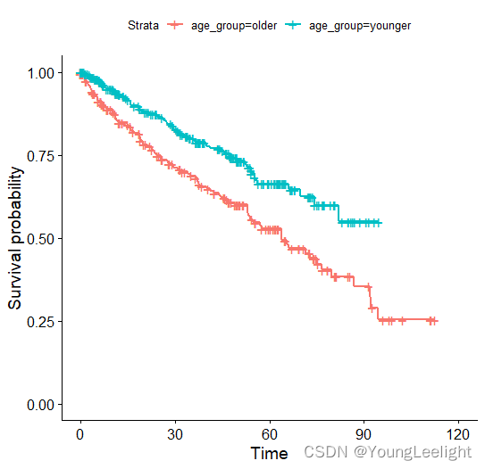

library(survival)
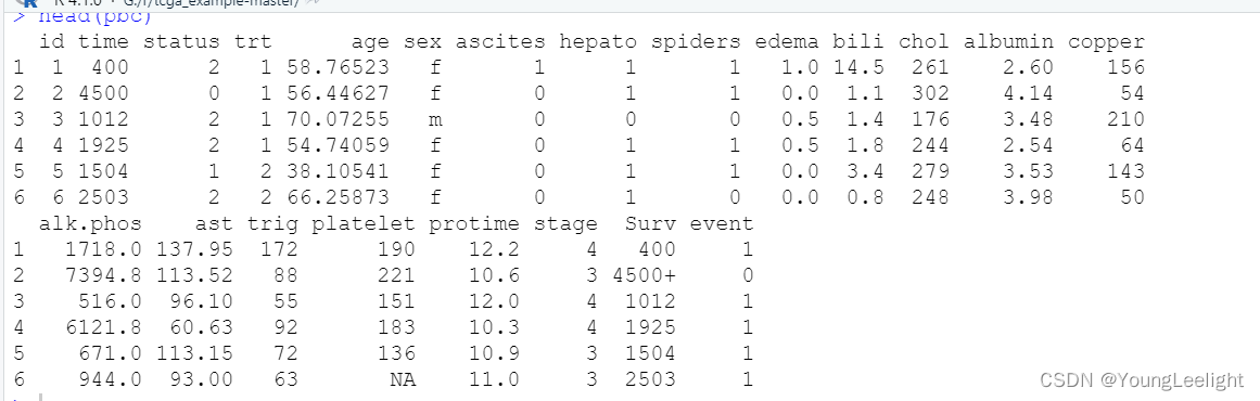
data(pbc)
pbc <- within(pbc, {## transplant (1) and death (2) are considered events, and marked 1event <- as.numeric(status %in% c(1,2))## Create a survival vectorSurv <- Surv(time, event)
})
head(pbc)

ggsurvplot(survfit(Surv ~ sex, data = pbc),                        label.curves = list(method = "arrow", cex = 1.2))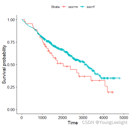

ggsurvplot(survfit(Surv ~ albumin >= median(albumin), data = pbc), label.curves = list(method = "arrow", cex = 1.2))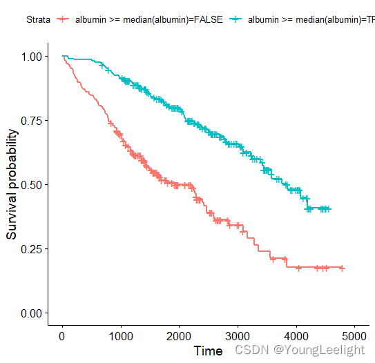

对五百多个miRNA基因进行批量运行cox，需要一点点时间。

如果是mRNA-seq的表达矩阵， 通常耗时更长。

注意，如果是某些基因表达量为恒定，比如在所有样本为0，这个代码会爆仓

需要去除这样的基因，没有分析的必要性。

exprSet[1:3,1:3]

#https://zhuanlan.zhihu.com/p/130316068

cox_results <-apply(exprSet , 1 , function(gene){

gene= exprSet[1,]

group=ifelse(gene>median(gene),‘high’,‘low’)
survival_dat <- data.frame(group=group,stage=phe$stage,age=phe$age, #新建存活矩阵，试图阐明某个基因的高低表达对生存率的影响
gender=phe$gender,
stringsAsFactors = F)
m=coxph(mySurv ~ gender + age + stage+ group, data = survival_dat) #矫正其他因素

beta <- coef(m)
se <- sqrt(diag(vcov(m)))
HR <- exp(beta)
HRse <- HR * se

#summary(m)
tmp <- round(cbind(coef = beta, se = se, z = beta/se, p = 1 - pchisq((beta/se)^2, 1),
HR = HR, HRse = HRse,
HRz = (HR - 1) / HRse, HRp = 1 - pchisq(((HR - 1)/HRse)^2, 1),
HRCILL = exp(beta - qnorm(.975, 0, 1) * se),
HRCIUL = exp(beta + qnorm(.975, 0, 1) * se)), 3)
return(tmp[‘grouplow’,])

})
cox_results=t(cox_results)
head(cox_results)
table(cox_results[,4]<0.05)
cox_results[cox_results[,4]<0.05,] #coxph 回归方法得到p<0.05的所有miRNA, 接下来与logrank test 得到的结果对比一下

批量生存分析 使用 logrank test 方法

mySurv=with(phe,Surv(time, event))
log_rank_p <- apply(exprSet , 1 , function(gene){

gene=exprSet[1,]

phe$group=ifelse(gene>median(gene){,}^{\prime }hig{h}^{\prime }{,}^{\prime }lo{w}^{\prime })data.survdiff=survdiff(mySurvgroup,data=phe)p.val=1-pchisq(data.survdiff$chisq, length(data.survdiff$n) - 1)
return(p.val)
})

require(“VennDiagram”)
VENN.LIST=list(cox=rownames(cox_results[cox_results[,4]<0.05,]),#coxph 回归方法得到p<0.05的所有miRNA
log=names(log_rank_p[log_rank_p<0.05])) #logrank test 得到的p<0.05的所有miRNA
venn.plot <- venn.diagram(VENN.LIST , NULL,
fill=c(“darkmagenta”, “darkblue”),
alpha=c(0.5,0.5), cex = 2,
cat.fontface=4,
main=“overlap of coxph and log-rank test”)

可以看到两种生存分析挑出来的基因重合度尚可。

grid.draw(venn.plot)

save(log_rank_p,cox_results ,
file =
file.path(Rdata_dir,‘TCGA-KIRC-miRNA-survival_results.Rdata’)
)

可以看到，文章里面挑选出来的生存分析相关的miRNA基因，在我们的分析里面都是显著的。