荟萃分析R Meta-Analyses 2----发现R

2.1安装R和R Studio

在开始之前，我们必须下载并准备一个计算机程序，该程序使我们能够方便地使用R进行统计分析。目前最好的选择可能是R Studio。该程序为我们提供了一个用户界面，使我们可以更轻松地处理数据、包和输出。最好的部分是 R Studio 完全免费，可以随时在 Internet 上下载。最近，R Studio 的在线版本已经发布，它通过网络浏览器为您提供基本相同的界面和功能。然而，在本书中，我们将重点关注直接安装在计算机上的 R Studio 版本。

在本章中，我们将重点介绍如何 在计算机上安装 R和 R Studio 。如果您已经在计算机上安装了 R Studio，并且您是经验丰富的R用户，那么这些对您来说可能都不陌生。那么你可以跳过这一章。如果您以前从未使用过R，请耐心等待。

让我们完成为我们的第一次编码工作设置R和 R Studio 的必要步骤。

R Studio 是一个允许我们编写R代码并以简单的方式运行它的界面。但 R Studio 与R并不相同；它要求您的计算机上已安装R软件。首先，我们必须安装最新的R版本。与 R Studio 一样，R是完全免费的。它可以从综合R档案网络（CRAN）网站下载。您必须下载的R类型取决于您使用的是Windows PC还是Mac。关于R 的一个重要细节是它的版本。R会定期更新，这意味着新版本可用。当您的R版本变得过于过时时，可能会出现某些功能不再起作用的情况。因此，通过重新安装R来定期（大约每年）更新R版本会很有帮助。对于本书，我们使用R版本 4.0.3。当您安装R时，可能已经有更高版本可用，建议始终安装最新版本。
下载并安装R后，您可以从R Studio 网站下载“R Studio Desktop” 。还有一些版本的 R Studio 需要您购买许可证，但这对于我们的目的来说绝对不是必需的。只需下载并安装 R Studio Desktop 的免费版本即可。
第一次打开 R Studio 时，它可能看起来很像图2.1所示。 R Studio 中有三个窗格。在右上角，我们有“环境”窗格，它显示我们在R内部定义（即保存）的对象。在右下角，您可以找到“文件”、“绘图”、“包”和“帮助”窗格。该窗格有多种功能；例如，它用于显示计算机上的文件、显示绘图和已安装的软件包以及访问帮助页面。然而，R Studio 的核心位于左侧，您可以在其中找到Console。控制台是所有R代码输入然后运行的地方。

R Studio 中的窗格。

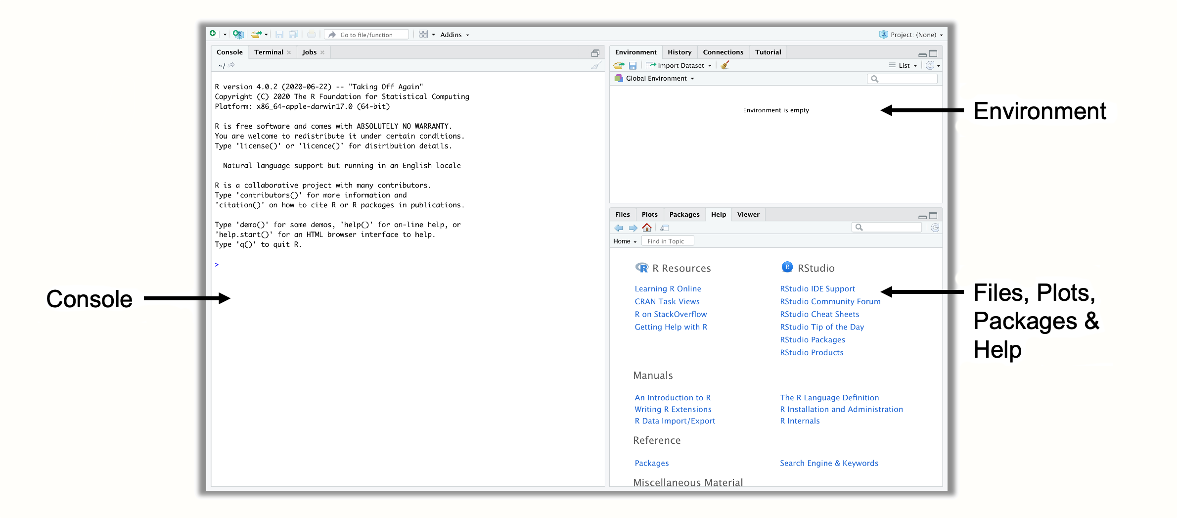
图 2.1：R Studio 中的窗格。

R Studio 中有第四个窗格，通常不会在开始时显示，即源窗格。您可以通过单击菜单中的“文件” > “新建文件” > “R 脚本”来打开源窗格。这将在左上角打开一个新窗格，其中包含一个空的R 脚本。R脚本是将代码收集到一个地方的好方法；您还可以将它们保存为计算机上扩展名为“.R”的文件（例如 myscript.R ）。要运行R脚本中的代码，请通过将光标拖过所有相关行来选择它，然后单击右侧的“运行”按钮。这会将代码发送到控制台，并在那里对其进行评估。快捷键是 Ctrl + R (Windows) 或 Cmd + R (Mac)。

2.2封装

我们现在将使用R代码安装一些软件包。包是R如此强大的主要原因之一。它们允许世界各地的专家开发其他人可以下载然后在R中使用的函数集。函数是R的核心元素；它们允许我们执行预定义类型的操作，通常是对我们自己的数据。

函数的数学公式与R中定义函数的方式之间存在相似之处。在R中，函数的编码方式是首先写下其名称，然后是包含函数的输入和/或规范（所谓的参数）的括号。F（X）�(�)

假设我们想知道 9 的平方根是多少。在R中，我们可以使用该sqrt函数来实现此目的。我们只需提供9函数的输入即可获得结果。你可以自己尝试一下。在控制台中的小箭头 ( >) 旁边，写下内容sqrt(9)，然后按 Enter 键。让我们看看会发生什么。

sqrt(9)## [1] 3

我们现在收到了R的第一个输出。它告诉我们 9 的平方根是 3。虽然R中的函数比这个复杂得多，但它们都遵循相同的原则：您提供函数所需的参数信息，函数使用此信息来进行计算，最后，它为您提供输出。

在Rinstall.packages中，我们还使用一个称为安装包的函数。我们唯一需要告诉这个函数的是我们想要安装的包的名称。目前，我们应该安装三个软件包，因为它们稍后会有所帮助。

{tidyverse}. The {tidyverse} package (Wickham et al. 2019) is not a single package, but actually a bundle of packages which make it easy to manipulate and visualize data in R. When we install the {tidyverse} package, this provides us with the {ggplot2}, {dplyr}, {tidyr}, {readr}, {purrr}, {stringr} and {forcats} package at the same time. Functions included in the tidyverse have become very popular in the R community in recent years, and are used by many researchers, programmers and data scientists. If you want to learn more about the tidyverse, you can visit its website.
{meta}. This package contains functions which make it easy to run different types of meta-analyses (Balduzzi, Rücker, and Schwarzer 2019). We will primarily focus on this package in the guide, because it is easy to use, well documented, and very versatile. More info on the {meta} package can be found on its website.
{metafor}. The {metafor} package (Viechtbauer 2010) is also dedicated to conducting meta-analyses, and a true powerhouse in terms of functionality. Since we will use this package at times in later chapters, and because {metafor} is used by the {meta} package for many applications, it is best to have it installed. The {metafor} package also has an excellent documentation for various meta-analysis-related topics.
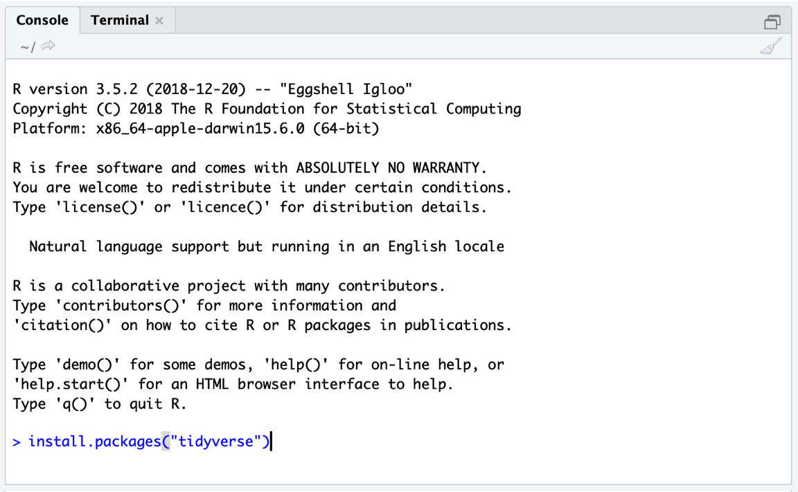
Figure 2.2: Installing a package.

The install.packages function only requires the name of the package we want to install as input. One package after another, our code should look like this:
```
install.packages("tidyverse")
install.packages("meta")
install.packages("metafor")
```
Simply type the code above into the console; then hit Enter to start the installation (see Figure 2.1).
不要忘记将包名称放入引号( "") 中。否则，您将收到错误消息。

按 Enter 键后，R将开始安装软件包并打印一些有关安装进度的信息。当install.packages函数完成后，包就可以使用了。安装的软件包被添加到R的系统库中。可以在R Studio 屏幕左下角的“包”窗格中访问该系统库。每当我们想要使用已安装的包时，我们都可以使用该library函数从我们的库中加载它。让我们尝试一下，并加载{tidyverse}包。
library(tidyverse)
2.3 { dmetar}包

在本指南中，我们希望使作为研究人员的您能够尽可能轻松地进行荟萃分析。尽管有像{meta}和{metafor}包这样出色的包可以完成大部分繁重的工作，但元分析的某些方面仍然是我们认为重要的，但目前在R中实现起来并不容易，特别是如果您这样做的话没有编程或统计背景。

为了填补这一空白，我们开发了{dmetar}包，它作为本书的配套R包。 {dmetar}包有自己的文档，可以在线找到。{dmetar}包的函数为{meta}和{metafor}包（以及其他一些更高级的包）提供了附加功能，我们将在本指南中经常使用它们。本书将详细介绍{dmetar}包中包含的大多数功能以及它们如何改进元分析工作流程。我们在本指南中使用的大多数示例数据集也包含在{dmetar}中。

尽管强烈推荐，但不一定要安装{dmetar}软件包才能完成本指南。对于包中的每个函数，我们还将提供源代码，可用于将函数保存在本地计算机上，以及这些函数所依赖的附加R包。我们还将提供包中包含的数据集的补充下载链接。
但是，预先安装{dmetar}软件包要方便得多，因为它会在您的计算机上预装所有功能和数据集。

要安装{dmetar}软件包，您计算机上的R版本必须为 3.6 或更高版本。如果您最近（重新）安装了R，则可能会出现这种情况。要检查您的R版本是否足够新，您可以将此行代码粘贴到控制台中，然后按 Enter 键。
```
R.Version()$version.string
```
This will display the current R version you have. If the R version is below 3.6, you will have to update it. There are good blog posts on the Internet providing guidance on how to do this.

If you want to install {dmetar}, one package already needs to be installed on your computer first. This package is called {devtools}. So, if {devtools} is not on your computer yet, you can install it like we did before.
```
install.packages("devtools")
```
You can then install {dmetar} using this line of code:
```
devtools::install_github("MathiasHarrer/dmetar")
```
This will initiate the installation process. It is likely that the installation will take some time because several other packages have to be installed along with the {dmetar} package for it to function properly. During the installation process, the installation manager may ask you if you want to update existing R packages on your computer. The output may look something like this:
```
## These packages have more recent versions available.
## Which would you like to update?
## 
## 1: All                          
## 2: CRAN packages only            
## 3: None                          
## 4: ggpubr (0.2.2 -> 0.2.3) [CRAN]
## 5: zip    (2.0.3 -> 2.0.4) [CRAN]
## 
## Enter one or more numbers, or an empty line to skip updates:
```
When you get this message, it is best to tell the installation manager that no packages should be updated. In our example, this means pasting 3 into the console and then hitting Enter. In the same vein, when the installation manager asks this question:
```
## There are binary versions available but the source versions are later:
##  
##  [...]
##  
##   Do you want to install from sources the package which needs compilation?
##   y/n: 
```
It is best to choose n (no). If the installation fails with this strategy (meaning that you get an Error), run the installation again, but update all packages this time.

When writing this book and developing the package, we made sure that everyone can install it without errors. Nevertheless, there is still a chance that installing the package does not work at the first try. If the installation problem persists, you can have a look at the “Contact Us” section in the Preface of this book.

2.4 Data Preparation & Import

This chapter will tell you how to import data into R using R Studio. Data preparation can be tedious and exhausting at times, but it is the backbone of all later steps. Therefore, we have to pay close attention to bringing the data into the correct format before we can proceed.

Usually, data imported into R is stored in Microsoft Excel spreadsheets first. We recommend to store your data there because this makes it very easy to do the import. There are a few “Dos and Don’ts” when preparing the data in Excel.
It is very important how you name the columns of your spreadsheet. If you already named the columns of your sheet adequately in Excel, you can save a lot of time later because your data does not have to be transformed using R. “Naming” the columns of the spreadsheet simply means to write the name of the variable into the first line of the column; R will automatically detect that this is the name of the column then.
Column names should not contain any spaces. To separate two words in a column name, you can use underscores or points (e.g. “column_name”).
It does not matter how columns are ordered in your Excel spreadsheet. They just have to be labeled correctly.
There is also no need to format the columns in any way. If you type the column name in the first line of your spreadsheet, R will automatically detect it as a column name.
It is also important to know that the import may distort special characters like ä, ü, ö, á, é, ê, etc. You might want to transform them into “normal” letters before you proceed.
Make sure that your Excel file only contains one sheet.
If you have one or several empty rows or columns which used to contain data, make sure to delete those columns/rows completely, because R could think that these columns contain (missing) data and import them also.

Let us start with an example data set. Imagine that you plan to conduct a meta-analysis of suicide prevention programs. The outcome you want to focus on in your study is the severity of suicidal ideation (i.e. to what degree individuals think about, consider, or plan to end their life), assessed by questionnaires. You already completed the study search and data extraction, and now want to import your meta-analysis data in R.

The next task is therefore to prepare an Excel sheet containing all the relevant data. Table 2.1 presents all the data we want to import. In the first row, this table also shows how we can name our columns in the Excel file based on the rules we listed above. We can see that the spreadsheet lists each study in one row. For each study, the sample size (n�), mean and standard deviation (SD��) is included for both the intervention and control group. This is the outcome data needed to calculate effect sizes, which is something we will cover in detail in Chapter 3. The following three columns contain variables we want to analyze later on as part of the meta-analysis.

We have prepared an Excel file for you called “SuicidePrevention.xlsx”, containing exactly this data. The file can be downloaded from the Internet.

Table 2.1: The suicide prevention dataset.
‘author’	‘n.e’	‘mean.e’	‘sd.e’	‘n.c’	‘mean.c’	‘sd.c’	‘pubyear’	‘age_group’	‘control’
	Intervention Group			Control Group			Subgroups
Author	N	Mean	SD	N	Mean	SD	Year	Age Group	Control Group
Berry et al.	90	14.98	3.29	95	15.54	4.41	2006	general	WLC
DeVries et al.	77	16.21	5.35	69	20.13	7.43	2019	older adult	no intervention
Fleming et al.	30	3.01	0.87	30	3.13	1.23	2006	general	no intervention
Hunt & Burke	64	19.32	6.41	65	20.22	7.62	2011	general	WLC
McCarthy et al.	50	4.54	2.75	50	5.61	2.66	1997	general	WLC
…	…	…	…	…	…	…	…	…	…

To import our Excel file in R Studio, we have to set a working directory first. The working directory is a folder on your computer from which R can use data, and in which outputs are saved. To set a working directory, you first have to create a folder on your computer in which you want all your meta-analysis data and results to be saved. You should also save the “SuicidePrevention.xlsx” file we want to import in this folder.

Then start R Studio and open your newly created folder in the bottom left Files pane. Once you have opened your folder, the Excel file you just saved there should be displayed. Then set this folder as the working directory by clicking on the little gear wheel on top of the pane, and then on Set as working directory in the pop-up menu. This will make the currently opened folder the working directory.

这将使当前打开的文件夹成为工作目录。

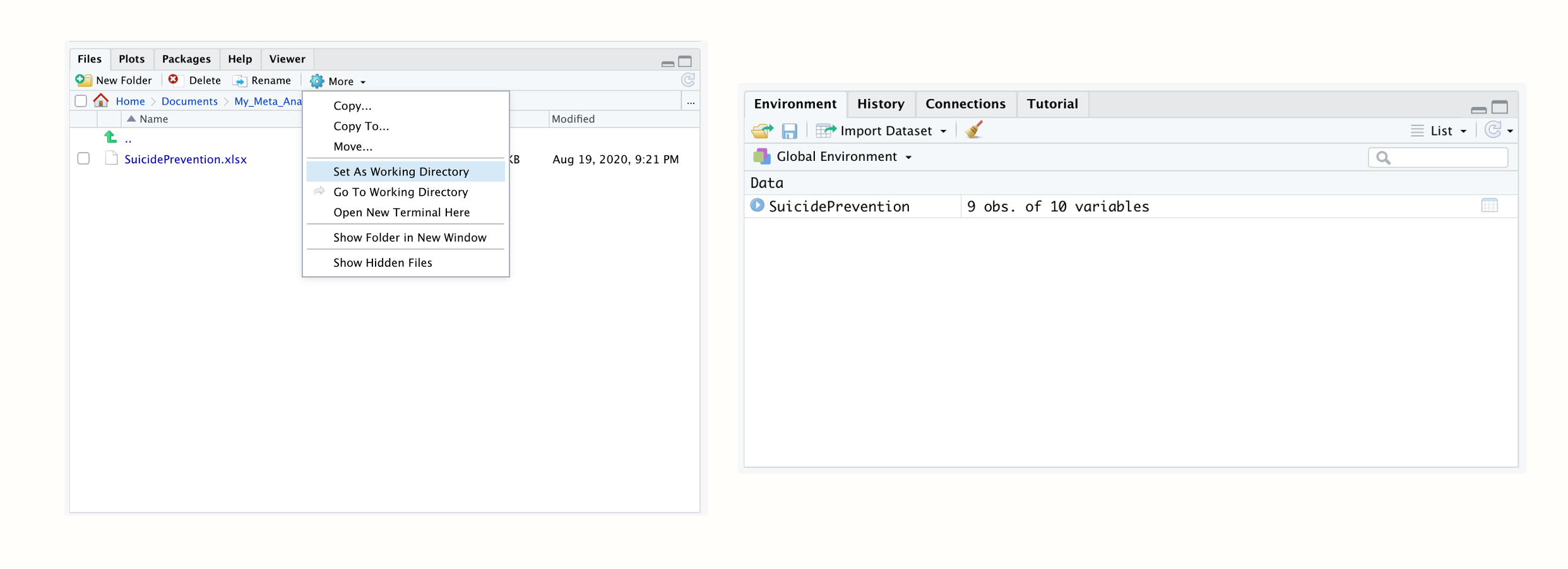
图2.3：设置工作目录； R环境中加载的数据集。

我们现在可以继续将数据导入到R中。在“文件”窗格中，只需单击“SuicidePrevention.xlsx”文件。然后单击导入数据集...。现在应该会弹出一个导入助手，它也会加载数据的预览。有时这可能很耗时，因此您可以根据需要跳过此步骤，然后直接单击“导入”。

然后，您的数据集及其名称应列SuicidePrevention在右上方的环境窗格中。这意味着您的数据现已加载并可供R代码使用。像我们在这里导入的表格数据集在R中称为数据框( data.frame) 。数据框是具有列和行的数据集，就像我们刚刚导入的Excel电子表格一样。

{openxlsx}

也可以直接使用代码导入数据文件。我们可以使用一个很好的包来执行此操作，称为{openxslx} ( Schauberger and Walker 2020 )。与所有R软件包一样，您必须先安装它。然后您可以使用该read.xlsx功能导入Excel工作表。

如果文件保存在您的工作目录中，您只需向函数提供文件名，并将导入的数据分配给R中的对象。例如，如果我们希望数据集具有Rdata中的名称，我们可以使用以下代码：
library(openxlsx)
data <- read.xlsx("SuicidePrevention.xlsx")
2.5数据操作

现在我们已经使用 R Studio 导入了第一个数据集，让我们进行一些操作。数据整理，意味着对数据进行转换以使其可用于进一步分析，是所有数据分析的重要组成部分。一些职业，例如数据科学家，花费大部分时间将原始的“杂乱”数据转变为“整齐”的数据集。{tidyverse}的函数为数据整理提供了一个出色的工具箱。如果您尚未从库中加载包，则应该立即为以下示例加载该包。

library(tidyverse)

2.5.1类转换

首先，我们应该看一下SuicidePrevention在上一章中导入的数据集。为此，我们可以使用{tidyverse}glimpse提供的函数。

glimpse(SuicidePrevention)
```
## Rows: 9
## Columns: 10
## $ author <chr> "Berry et al.", "DeVries et al.", "Fleming et al.", "Hunt & …
## $ n.e <chr> "90", "77", "30", "64", "50", "109", "60", "40", "51"
## $ mean.e <chr> "14.98", "16.21", "3.01", "19.32", "4.54", "15.11", "3.44", …
## $ sd.e <chr> "3.29", "5.35", "0.87", "6.41", "2.75", "4.63", "1.26", "0.7…
## $ n.c <dbl> 95, 69, 30, 65, 50, 111, 60, 40, 56
## $ mean.c <chr> "15.54", "20.13", "3.13", "20.22", "5.61", "16.46", "3.42", …
## $ sd.c <chr> "4.41", "7.43", "1.23", "7.62", "2.66", "5.39", "1.88", "1.4…
## $ pubyear <dbl> 2006, 2019, 2006, 2011, 1997, 2000, 2013, 2015, 2014
## $ age_group <chr> "general", "older adult", "general", "general", "general", "…
## $ control <chr> "WLC", "no intervention", "no intervention", "WLC", "WLC", "…
```
我们看到，这为我们提供了有关数据集每列中存储的数据类型的详细信息。有不同的缩写表示不同类型的数据。在R中，它们被称为类。

<num>代表数字.这是所有以数字形式存储的数据（例如 1.02）。

<chr>代表性格。这是以单词形式存储的所有数据。

我们还可以使用该函数检查列的类class。我们可以通过将$运算符添加到其名称，然后添加列的名称来直接访问数据框中的列。让我们试试这个。首先，我们让R为我们提供列中包含的数据n.e。之后，我们检查列的类别。
- <log>代表逻辑。这些是二元变量，这意味着它们表示条件是TRUE或FALSE。
- <factor>代表因子.因子存储为数字，每个数字表示变量的不同级别。变量的可能因子水平可能为 1 =“低”、2 =“中”、3 =“高”。
我们检查列的类别。
```
SuicidePrevention$n.e## [1] "90" "77" "30" "64" "50" "109" "60" "40" "51"
```
```
class(SuicidePrevention$n.e)## [1] "character"
```
我们看到包含干预组样本量的列的n.e类别为character。但是等等，那是错误的类！在导入过程中，该列被错误地分类为character变量，而它实际上应该具有类numeric。这对进一步的分析步骤有影响。例如，如果我们想计算平均样本量，我们会收到以下警告：
```
mean(SuicidePrevention$n.e)## Warning in mean.default(SuicidePrevention$n.e): argument is not numeric or
## logical: returning NA
```
```
## [1] NA
```
为了使我们的数据集可用，我们通常必须首先将列转换为正确的类。为此，我们可以使用一组均以“ as.”开头的函数： as.numeric、as.character和。让我们看几个例子。as.logicalas.factor

glimpse在之前函数的输出中，我们看到有几列已被赋予character类，而它们应该是numeric。这涉及列n.e、mean.e、sd.e和mean.c。sd.c我们看到出版年份pubyear有class <dbl>。这代表double，意味着该列是一个数值向量。在R中使用double和来指代数字数据类型是一个历史异常现象。然而，通常这没有实际意义。numeric

然而，某些数值在我们的数据集中被编码为字符这一事实将导致下游出现问题，因此我们应该使用该as.numeric函数更改类。我们为函数提供要更改的列，然后使用赋值运算符( <-) 将输出保存回其原始位置。这导致以下代码。

SuicidePrevention$n.e <- as.numeric(SuicidePrevention$n.e)
SuicidePrevention$mean.e <- as.numeric(SuicidePrevention$mean.e)
SuicidePrevention$sd.e <- as.numeric(SuicidePrevention$sd.e)
SuicidePrevention$n.c <- as.numeric(SuicidePrevention$n.c)
SuicidePrevention$mean.c <- as.numeric(SuicidePrevention$mean.c)
SuicidePrevention$sd.c <- as.numeric(SuicidePrevention$sd.c)
SuicidePrevention$n.c <- as.numeric(SuicidePrevention$n.c)

我们还在glimpse输出中看到，数据中的子组age_group和被编码为字符。control然而，实际上，将它们编码为因子更合适，每个因子有两个级别

我们还在glimpse输出中看到，数据中的子组age_group和被编码为字符。control然而，实际上，将它们编码为因子更合适，每个因子有两个级别。我们可以使用该as.factor函数来更改类。
```
<code>SuicidePrevention$age_group <- <a data-cke-saved-href="https://rdrr.io/r/base/factor.html" href="https://rdrr.io/r/base/factor.html">as.factor</a>(SuicidePrevention$age_group)
SuicidePrevention$control <- <a data-cke-saved-href="https://rdrr.io/r/base/factor.html" href="https://rdrr.io/r/base/factor.html">as.factor</a>(SuicidePrevention$control)</code>
```
使用levelsandnlevels函数，我们还可以查看因子标签和因子中的级别数。
```
<code><a data-cke-saved-href="https://rdrr.io/r/base/levels.html" href="https://rdrr.io/r/base/levels.html">levels</a>(SuicidePrevention$age_group)</code>
```
```
## [1] "general" "older adult"
```
```
<code><a data-cke-saved-href="https://rdrr.io/r/base/nlevels.html" href="https://rdrr.io/r/base/nlevels.html">nlevels</a>(SuicidePrevention$age_group)</code>
```
```
## [1] 2
```
我们还可以使用该levels函数来更改因子标签的名称。我们只需为原始标签分配新名称即可。要在R中执行此操作，我们必须使用concatenate , orc函数。此函数可以将两个或多个单词或数字连接在一起并创建一个元素。让我们试试这个。
```
SuicidePrevention$age_group <- as.factor(SuicidePrevention$age_group)
SuicidePrevention$control <- as.factor(SuicidePrevention$control)
```
```
levels(SuicidePrevention$age_group)
```
```
## [1] "gen" "older"
```
完美的。我们现在可以使用新创建的new.factor.levels对象并将其分配给列的因子标签age_group。

levels(SuicidePrevention$age_group) <- new.factor.levels

让我们检查一下重命名是否有效。

SuicidePrevention$age_group
```
## [1] gen older gen gen gen gen gen older older
## Levels: gen older
```
还可以使用创建逻辑as.logical。假设我们想要重新编码该列pubyear，以便它仅显示 2009 年之后发布的研究。为此，我们必须通过代码定义是/否规则。我们可以使用“大于或等于”运算符来完成此操作>=，然后将其用作函数的输入as.logical。
```
SuicidePrevention$pubyear
```
```
## [1] 2006 2019 2006 2011 1997 2000 2013 2015 2014
```
```
as.logical(SuicidePrevention$pubyear >= 2010)
```
```
## [1] FALSE TRUE FALSE TRUE FALSE FALSE TRUE TRUE TRUE
```
我们可以看到，这对pubyearasTRUE或中的每个元素进行编码FALSE，具体取决于出版年份是否大于或等于 2010 年。
2.5.2数据切片

在R中，有多种方法可以提取数据帧的子集。我们已经介绍了一种方法，即$运算符，它可用于提取列。从数据集中提取切片的更通用方法是使用方括号。使用方括号时我们必须遵循的通用形式是data.frame[rows, columns]。始终可以使用行和列在数据集中出现的数字来提取行和列。例如，我们可以使用下面的代码来提取数据框第二行的数据。
```
SuicidePrevention[2,]
```

##           author n.e mean.e sd.e n.c mean.c sd.c pubyear age_group
## 2 DeVries et al.  77  16.21 5.35  69  20.13 7.43    2019     older
##           control
## 2 no intervention

我们可以更具体地告诉R我们只需要第二行第一列中的信息。

SuicidePrevention[2, 1]

## [1] "DeVries et al."

要选择特定的切片，我们必须c再次使用 concatenate ( ) 函数。例如，如果我们想要提取第2行和第3行以及第4行和第6列，我们可以使用此代码。

SuicidePrevention[c(2,3), c(4,6)]

##   sd.e mean.c
## 2 5.35  20.13
## 3 0.87   3.13

通常只能按行号选择行。但是，对于列，也可以提供列名称而不是数字。

SuicidePrevention[, c("author", "control")]

##            author         control
## 1    Berry et al.             WLC
## 2  DeVries et al. no intervention
## 3  Fleming et al. no intervention
## 4    Hunt & Burke             WLC
## 5 McCarthy et al.             WLC
## 6   Meijer et al. no intervention
## 7   Rivera et al. no intervention
## 8  Watkins et al. no intervention
## 9  Zaytsev et al. no intervention

另一种可能性是根据行值过滤数据集。我们可以使用该filter函数来做到这一点。在函数中，我们需要指定数据集名称以及过滤逻辑。一个相对简单的例子是过滤所有n.e等于或小于 50 的研究。

filter(SuicidePrevention, n.e <= 50)

##            author n.e mean.e sd.e n.c mean.c sd.c pubyear age_group
## 1  Fleming et al.  30   3.01 0.87  30   3.13 1.23    2006       gen
## 2 McCarthy et al.  50   4.54 2.75  50   5.61 2.66    1997       gen
## 3  Watkins et al.  40   7.10 0.76  40   7.38 1.41    2015     older
##           control
## 1 no intervention
## 2             WLC
## 3 no intervention

但也可以按名称过滤。想象一下，我们想要提取作者Meijer和Zaytsev的研究。为此，我们必须使用%in%运算符和连接函数定义过滤逻辑。

filter(SuicidePrevention, author %in% c("Meijer et al.",
"Zaytsev et al."))

##           author n.e mean.e sd.e n.c mean.c  sd.c pubyear age_group
## 1  Meijer et al. 109  15.11 4.63 111  16.46  5.39    2000       gen
## 2 Zaytsev et al.  51  23.74 7.24  56  24.91 10.65    2014     older
##           control
## 1 no intervention
## 2 no intervention

相反，我们也可以通过在过滤逻辑前面加上感叹号来提取除Meijer和Zaytsev之外的所有研究。

filter(SuicidePrevention, !author %in% c("Meijer et al.",
"Zaytsev et al."))

2.5.3数据转换

当然，也可以更改R数据框中的特定值，或扩展它们。要更改R内部保存的数据，我们必须使用赋值运算符。让我们重新使用之前学到的有关数据切片的知识来更改数据集中的特定值。想象一下，我们犯了一个错误，德弗里斯等人的研究的发表年份。被错误地报告为 2019 年，而实际上应该是 2018 年。我们可以通过相应地切片数据集来更改该值，然后分配新值。请记住DeVries 等人的结果。在数据集的第二行中报告。

SuicidePrevention[2, "pubyear"] <- 2018
SuicidePrevention[2, "pubyear"]

## [1] 2018

也可以一次更改多个值。例如，如果我们想要为数据集中的每个干预组均值添加 5，我们可以使用此代码来实现。

SuicidePrevention$mean.e + 5

## [1] 19.98 21.21  8.01 24.32  9.54 20.11  8.44 12.10 28.74

我们还可以使用两个或更多列来进行计算。一个实际相关的例子是，我们可能有兴趣计算每项研究的干预组和对照组平均值之间的平均差异。与其他编程语言相比，这在R中非常容易。

SuicidePrevention$mean.e - SuicidePrevention$mean.c

## [1] -0.56 -3.92 -0.12 -0.90 -1.07 -1.35  0.02 -0.28 -1.17

正如您所看到的，这取每项研究的干预组平均值，然后减去对照组平均值，每次都使用同一行的值。想象一下我们稍后想要使用这个均值差。因此，我们希望将其保存为一个名为的额外对象md，并将其作为新列添加到我们的SuicidePrevention数据框中。使用赋值运算符两者都很容易。

md <- SuicidePrevention$mean.e - SuicidePrevention$mean.c

SuicidePrevention$md <- SuicidePrevention$mean.e -
SuicidePrevention$mean.c

我们想向您展示的最后一件事是管道操作员。在R中，管道写为%>%。管道本质上允许我们将函数应用于对象，而不必直接在函数调用中指定对象名称。我们只需使用管道运算符连接对象和函数。让我们给你一个简单的例子。如果我们想计算对照组中的平均样本量，我们可以使用该mean函数和管道运算符，如下所示：

SuicidePrevention$n.c %>% mean()

## [1] 64

诚然，在这个例子中，很难看出这种管道的附加值。管道的特殊优势在于它们允许我们将许多功能链接在一起。想象一下，我们想知道对照组样本量平均值的平方根，但仅限于 2009 年之后发表的研究。管道让我们可以轻松地一步完成此操作。

SuicidePrevention %>%
filter(pubyear > 2009) %>%
pull(n.c) %>%
mean() %>%
sqrt()
## [1] 7.615773
在管道中，我们使用了一个之前没有涉及过的函数，即函数pull。这个函数可以看作是$我们在管道中使用的运算符的等价物。它只是“拉出”我们在函数中指定的变量，因此可以将其转发到管道的下一部分。

访问R文档

R 中的许多函数需要多个参数，并且不可能记住如何正确使用所有函数。值得庆幸的是，没有必要熟记每个函数是如何使用的。 R Studio使我们可以轻松访问R文档，其中每个函数都有详细的描述页面。

有两种方法可以搜索函数文档页面。第一种方法是访问R Studio 左下角的“帮助”窗格，然后使用搜索栏查找有关特定函数的信息。更方便的方法是简单地运行，? 然后在控制台中输入函数名称，例如 ?mean。这将自动打开该函数的文档条目。

函数的R 文档通常至少包含“用法”、“参数”和 “示例”部分。参数和示例部分通常对于理解函数的使用方式特别有帮助。

2.5.4保存数据

一旦我们对数据进行了转换并将其保存在R内部，我们就必须在某个时候将其导出。我们建议您在保存R数据帧时使用两种类型的文件格式： .rda和.csv。

以.rda结尾的文件代表R Data。它是专门针对R 的文件类型，具有所有优点和缺点。.rda文件的优点是可以轻松地在R中重新打开它们，并且不存在数据在导出过程中可能被扭曲的风险。它们的用途也非常广泛，可以保存不适合电子表格格式的数据。缺点是只能在R中打开；但对于某些项目来说，这已经足够了。

要将对象另存为.rda数据文件，您可以使用该save函数。在该函数中，您必须提供 (1) 对象的名称，以及 (2)您希望文件具有的确切名称，包括文件结尾。运行该函数会将文件保存到您的工作目录中。

save(SuicidePrevention, file = "suicideprevention.rda")

以.csv结尾的文件代表逗号分隔值。一般来说，这种格式是最常用的数据格式之一。它可以由许多程序打开，包括Excel。您可以使用该write.csv函数将数据保存为.csv。代码结构和行为与的代码结构和行为几乎相同save，但提供的对象需要是数据框或其他表格数据对象。当然，您需要指定文件类型“.csv”。

write.csv(SuicidePrevention, file = "suicideprevention.csv")

这只是R中数据操作策略的快速概述。从头开始学习R有时会让人筋疲力尽，尤其是当我们处理像操作数据这样简单的事情时。然而，习惯R工作方式的最佳方法是练习。一段时间后，常见的R命令将成为您的第二天性。

继续学习的一个好方法是查看 Hadley Wickham 和 Garrett Grolemund 的书《R for Data Science》 （2016 年）。与本指南一样，这本书可以完全免费在线阅读。此外，我们还在下一页收集了一些练习，您可以用它们来练习我们在这里学到的知识。

■◼

2.6问题与解答

数据操作练习

对于这些练习，我们将使用一个名为的新数据集 data。您可以使用以下代码直接在R中创建此数据集：

data <- data.frame("Author" = c("Jones", "Goldman",
"Townsend", "Martin",
"Rose"),
"TE" = c(0.23, 0.56,
0.78, 0.23,
0.33),
"seTE" = c(0.324, 0.235,
0.394, 0.275,
0.348),
"subgroup" = c("one", "one",
"two", "two",
"three"))

以下是该数据集的练习。