实例10: 四足机器人运动学逆解单腿可视化
实验目的
- 了解逆运动学的有无解、有无多解情况。
- 了解运动学逆解的求解。
- 熟悉逆运动学中求解的几何法和代数法。
- 熟悉单腿舵机的简单校准。
- 掌握可视化逆向运动学计算结果的方法。
实验要求
- 拼装一条mini pupper的腿部。
- 运行程序,可视化观察运动学逆解的多解情况和求解方法。
- 对单腿舵机进行简单校准。
- 观察运动学逆解的硬件运行情况。
实验知识
1.什么是逆向运动学 Inverse Kinematics
正向运动学探究的是已知关节角θi\theta_iθi,求解工具坐标系{H}\{H\}{H}或WorldP^{World}PWorldP的问题。
而逆向运动学则是探究已知工具坐标系{H}\{H\}{H}的位置和姿态或WorldP^{World}PWorldP,求解满足要求的θi\theta_iθi的问题。
运动学方程解的有无定义了工作空间,有解则表示机械臂能到达这个目标点,无解则表示机械臂无法到达这个点,这个目标点位于工作空间之外。
基本的逆运动学可以看做是给定操作臂末端执行器的位置和姿态,计算所有可达给定位置和姿态的关节角的问题,可以认为是机器人位姿从笛卡尔空间到关节空间的“定位”映射。
2.什么是封闭解和数值解
逆运动学不像正运动学那么容易,逆运动学是非线性的,难以找到封闭解,有时候无解,有时候有有多解的问题,这种非线性的超越方程组,没有规矩的、统一、通用的解法,解法分为封闭解法和数值解法。
封闭解是由数学公式的推导得出,对于任意自变量均能求出对应的因变量,计算量可能相对较多,精度高。
数值解则是可以由离散查表或者是插值一类的方法去模拟最终情况,计算量相对较小,精度相对较差。
因此,我们需要根据实际情况来考虑逆向运动学的解和解的情况。
2.解存在吗?
在逆向运动学(IK)中,我们可以通过给定点相对于世界坐标系(Frame World)的坐标来解算出机器人的手臂关节应该旋转的角度θ\thetaθ。
假如给定的一个位置是在很远的地方,机器人的手臂完全够不着,那么求解是没有意义的,因此我们将会用到工作空间来描述机器人可触达的区域。
工作空间
工作空间是手臂末端所能到达的位置范围。指定的目标点必须在工作空间内,逆向运动学求解才有意义。
为了进一步描述工作空间,可以用以下常见的这两种工作空间的表示:
可达工作空间 Reachable workspace
是手臂能用一种或以上的姿态能够到达的位置范围。可达目标坐标系可以描述这个Frame相对于世界坐标系的位置,而一系列的可达目标坐标系的集合构成了可达工作空间。
灵巧工作空间 Dexterous workspace
是手臂末端用任何姿态都能够到达的位置,条件相当苛刻,比如平面2DOFs的RR机械臂模型中L1=L2的摆臂的圆心,在这个模型中,仅此一点是灵巧工作空间。灵巧工作空间是可达工作空间的子集。
3.是否有多个解?
在求解运动学方程时常常会遇到不只一个解的情况。比如平面中具有三个旋转关节的机器人手臂,对于同一个点PPP,这三个旋转关节可以有不同的位形,在不同的位型下,手臂末端的执行器的可达位置和姿态可以是相同的。
图片:三连杆操作臂多解图
解的选取
对于解的选取有一些基本原则:
- 速度最快
- 能耗最低
- 避开障碍物
- 在关节允许活动的范围限制内
4.如何求解?
求解操作臂运动学方程是非线性的问题,非线性方程组没有通用的求解算法,算法需要针对机器人手臂的模型来制定。如果某一算法可以解出与已知位姿相关的全部关节变量,那么这个机器人手臂就是可解的。
从Frameobject{Frame_{object}}Frameobject到FrameWorld{Frame_{World}}FrameWorld的变换矩阵oWT^W_oToWT中的转动部分和平移部分可以提取出含未知数的16个数字。
其中的旋转矩阵被xyz相互垂直、xyz为单位向量这六个条件限制到只有三个自由度,其中的位置矢量分量的三个方程有三个自由度,共有6个限制条件,6个自由度,这些方程为非线性超越方程,求解不易。
对于六旋转关节的机械臂,存在解析解(封闭解)的充分条件是相邻的三关节的转轴交于一点。
60T=[60R3x30P6ORG3x10001]4x4=[X^6⋅X^0Y^6⋅X^0Z^6⋅X^060PXorgX^6⋅Y^0Y^6⋅Y^0Z^6⋅Y^060PYorgX^6⋅Z^0Y^6⋅Z^0Z^6⋅Z^060PZorg0001]^0_6T = \left[ \begin{matrix} ^0_6R_{3x3} &^0P_{6{\kern 2pt}ORG{\kern 2pt}3x1}\\ 0{\kern 3pt}0{\kern 3pt}0&1 \end{matrix} \right]_{4x4}= \left[ \begin{matrix} \hat X_6\cdot \hat X_0& \hat Y_6\cdot \hat X_0 & \hat Z_6\cdot \hat X_0 & ^0_6P_{Xorg}\\ \hat X_6\cdot \hat Y_0& \hat Y_6\cdot \hat Y_0&\hat Z_6\cdot \hat Y_0 &^0_6P_{Yorg}\\ \hat X_6\cdot \hat Z_0& \hat Y_6\cdot \hat Z_0&\hat Z_6\cdot \hat Z_0 &^0_6P_{Zorg}\\ 0&0&0&1 \end{matrix} \right] 60T=[60R3x30000P6ORG3x11]4x4=X^6⋅X^0X^6⋅Y^0X^6⋅Z^00Y^6⋅X^0Y^6⋅Y^0Y^6⋅Z^00Z^6⋅X^0Z^6⋅Y^0Z^6⋅Z^0060PXorg60PYorg60PZorg1
对于基于解析形式的解法,常见的求解方法有几何法和代数法。两种方法相似,求解过程不同。
几何法
几何法求解机械臂的逆运动学问题时,常常需要将空间几何参数转化为平面几何的问题。在αi=0或−+90°\alpha_i=0 或 ^+_-90°αi=0或−+90°时几何法会非常容易,应用平面几何常见的公式及角度转换即可求出θi\theta_iθi的值。
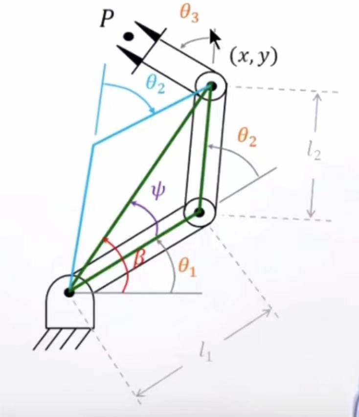
x2+y2=l12+l22−2l1l2(π−θ2)(余弦定理)x^2+y^2=l^2_1+l^2_2-2l_1l_2(\pi-\theta_2) \tag{余弦定理} x2+y2=l12+l22−2l1l2(π−θ2)(余弦定理)
Cosθ2=x2+y2−l12−l222l1l2(变形1)Cos\theta_2={x^2+y^2-l^2_1-l^2_2\over 2l_1l_2} \tag{变形1} Cosθ2=2l1l2x2+y2−l12−l22(变形1)
Cosψ=(x2+y2)+l12−l222l1x2+y2(变形2)Cos\psi={(x^2+y^2)+l^2_1-l^2_2\over 2l_1\sqrt{x^2+y^2}} \tag{变形2} Cosψ=2l1x2+y2(x2+y2)+l12−l22(变形2)
θ1={atan2(y,x)+ψθ2<0atan2(y,x)−ψθ2>0\theta_1= \begin{cases} atan2(y,x)+\psi& \theta_2<0\\ atan2(y,x)-\psi& \theta_2>0\\ \end{cases} θ1={atan2(y,x)+ψatan2(y,x)−ψθ2<0θ2>0
在计算完θ2\theta_2θ2和θ1\theta_1θ1后,根据图的几何角度关系,又可算得θ3\theta_3θ3,即成功反解运动学的各θn\theta_nθn
math.atan2()方法
math.atan2()方法是双变量反正切公式,可以计算给定y,x值的反正切值,也就是以弧度形式表达的该段终点与起点连线斜率线的一个角度值。
atan2()优于atan(),因为可以计算x2-x1=0的情况。
参考链接:Python math.atan2(y,x)
计算空间中缺少的自由度
代数法
应用连杆参数(αi−1\alpha_{i-1}αi−1,ai−1a_{i-1}ai−1,θi\theta_{i}θi,did_{i}di),通过运动学正解(FK)可以求得机械臂的运动学方程,表现形式为变换矩阵30T^0_3T30T。因此,目标点的位置是由手臂末端坐标系相对基坐标系来定的,当研究对象为平面机械臂时,只需要知道x,y,ϕ\phiϕ即可确定目标点位置。
ϕ\phiϕ是 末端杆在平面内的姿态角
将已知的30T^0_3T30T与新建立的objectworldT^{world}_{object}TobjectworldT取等,即可获得对应位置的值相等。
[c123−s1230.0l1c1+l2c12s123c1230.0l1s1+l2s120.00.01.00.00001]=[cϕ−sϕ0.0xsϕcϕ0.0y0.00.01.00.00001]\left[ \begin{matrix} c_{123} & -s_{123} & 0.0&l_1c_1+l_2c_{12} \\ s_{123} & c_{123} & 0.0&l_1s_1+l_2s_{12} \\ 0.0 & 0.0 & 1.0 &0.0 \\ 0 & 0 & 0 &1 \\ \end{matrix} \right]= \left[ \begin{matrix} c_{\phi} & -s_{\phi} & 0.0&x \\ s_{\phi} & c_{\phi} & 0.0&y \\ 0.0 & 0.0 & 1.0 &0.0 \\ 0 & 0 & 0 &1 \\ \end{matrix} \right] c123s1230.00−s123c1230.000.00.01.00l1c1+l2c12l1s1+l2s120.01=cϕsϕ0.00−sϕcϕ0.000.00.01.00xy0.01
利用三角函数和角公式
Sin1−+2=Sin1Cos2−+Cos1Sin2Sin_{1 {^+_-}2}=Sin_1Cos_2 {^+_-} Cos_1Sin_2 Sin1−+2=Sin1Cos2−+Cos1Sin2
Cos1−+2=Cos1Cos2+−Sin1Sin2Cos_{1 {^+_-}2}=Cos_1Cos_2 {^-_+}Sin_1Sin_2 Cos1−+2=Cos1Cos2+−Sin1Sin2
可得
Cosθ2=x2+y2−l12−l222l1l2Cos\theta_2={x^2+y^2-l^2_1-l^2_2\over 2l_1l_2} Cosθ2=2l1l2x2+y2−l12−l22
此式在1≥Cosθ2≥−11\geq Cos\theta_2\geq-11≥Cosθ2≥−1时有解
假设目标点在工作空间内,又有
Sinθ2=−+1−c2Sin\theta_2= {^+_-}\sqrt {1-c^2} Sinθ2=−+1−c2
应用几何法中提到的math.Atan2()求解θ2\theta_2θ2,利用θ2\theta_2θ2再去对其他θn\theta_nθn求解,具体方法参考教材,本处仅作代数法引入。
通俗的来说,就是确认θn\theta_nθn的SinθnSin\theta_nSinθn和CosθnCos\theta_nCosθn,再利用双变量反正切公式math.Atan2()求θn\theta_nθn
实验步骤
1.逆运动学的多解与求解
运行程序,观察运动学逆解的多解情况,观察程序中运动学逆解的求解方法。
sudo python rr_IK.py
# 示例值: 3 7
#!/usr/bin/python
# coding:utf-8
# rr_IK.py
# 逆向运动学IK
# mini pupper的简化单腿,可视作同一平面的RR类机械臂,可视化该机械臂,由给定末端位置计算转轴角度
import matplotlib.pyplot as plt  # 引入matplotlib
import numpy as np  # 引入numpy
from math import degrees, radians, sin, cos# 几何法:端点坐标转关节角
def position_2_theta(x, y, l1, l2):"""运动学逆解 将输入的端点坐标转化为对应的关节角:param x: p点坐标x值:param y: p点坐标y值:param l1: 大臂长:param l2: 小臂长:return: 关节角1值1 关节角1值2 关节角2值1 关节角2值1"""cos2 = (x ** 2 + y ** 2 - l1 ** 2 - l2 ** 2) / (2 * l1 * l2)# print(cos2)sin2_1 = np.sqrt(1 - cos2 ** 2)sin2_2 = -sin2_1# print(sin2_1)# print("sin2有两值,分别为sin2_1=%f, sin2_2=%f" % (sin2_1, sin2_2))  # 若考虑关节情况也可只取一个正值theta2_1 = np.arctan2(sin2_1, cos2)theta2_2 = np.arctan2(sin2_2, cos2)phi_1 = np.arctan2(l2 * sin2_1, l1 + l2 * cos2)phi_2 = np.arctan2(l2 * sin2_2, l1 + l2 * cos2)theta1_1 = np.arctan2(y, x) - phi_1theta1_2 = np.arctan2(y, x) - phi_2# print(degrees(theta1_1), degrees(theta1_2), degrees(theta2_1), degrees(theta2_2))return theta1_1, theta1_2, theta2_1, theta2_2def preprocess_drawing_data(theta1, theta2, l1, l2):"""处理角度数据,转化为matplotlib适应的绘图格式:param theta1: 角度数据1:param theta2: 角度数据2:param l1: 杆件长1:param l2: 杆件长2:return: 绘图数据x坐标list和对应的y坐标list"""xs = [0]ys = [0]# 分别算出x1 y1和x2 y2x1 = l1 * cos(theta1)y1 = l1 * sin(theta1)x2 = x1 + l2 * cos(theta1 + theta2)y2 = y1 + l2 * sin(theta1 + theta2)xs.append(x1)xs.append(x2)ys.append(y1)ys.append(y2)return xs, ysdef annotate_angle(x0, y0, rad1, rad2, name, inverse=False):"""为两条直线绘制角度:param x0: 圆心x坐标:param y0: 圆心x坐标:param rad1: 起始角:param rad2: 终止角:param name: 角名:param inverse: 用于解决点1的重叠问题:return: 无"""theta = np.linspace(rad1, rad2, 100)  # 0~radr = 0.2  # circle radiusx1 = r * np.cos(theta) + x0y1 = r * np.sin(theta) + y0plt.plot(x1, y1, color='red')plt.scatter(x0, y0, color='blue')degree = degrees((rad2 - rad1))if inverse:plt.annotate("%s=%.1f°" % (name, degree), [x0, y0], [x0 - r / 1.5, y0 - r / 1.5])else:plt.annotate("%s=%.1f°" % (name, degree), [x0, y0], [x0 + r / 1.5, y0 + r / 1.5])# 关节信息
# 大臂长度:5 cm 小臂长度:7.5 cm
link_length = [5, 7.5]  # in cm
# 输入末端位置
position_pre = input("请输入末端的x坐标和y坐标,以空格隔开:")
position = [float(n) for n in position_pre.split()]
print(position)# 计算并预处理绘图数据
joints_angles = position_2_theta(position[0], position[1], link_length[0], link_length[1])
# print(joints_angles)
figure1 = preprocess_drawing_data(joints_angles[0], joints_angles[2], link_length[0], link_length[1])
figure2 = preprocess_drawing_data(joints_angles[1], joints_angles[3], link_length[0], link_length[1])
# print(figure1)
# print(figure2)# 绘图
fig, ax = plt.subplots()  # 建立图像
plt.axis("equal")
ax.grid()
plt.plot(figure1[0], figure1[1], color='black', label='method 1')
plt.scatter(figure1[0], figure1[1], color='black')
plt.plot(figure2[0], figure2[1], color='red', label='method 2')
plt.scatter(figure2[0], figure2[1], color='blue')
ax.set(xlabel='X', ylabel='Y', title='mini pupper IK RR model')
plt.legend()
# 标注
annotate_angle(figure1[0][0], figure1[1][0], 0, joints_angles[0], "theta1_1")
annotate_angle(figure1[0][1], figure1[1][1], joints_angles[0], joints_angles[2]+joints_angles[0], "theta2_1")
annotate_angle(figure2[0][0], figure2[1][0], 0, joints_angles[1], "theta1_2", inverse=True)
annotate_angle(figure2[0][1], figure2[1][1], joints_angles[1], joints_angles[3]+joints_angles[1], "theta2_2")
plt.annotate("P(%d, %d)" % (position[0], position[1]), [figure1[0][2], figure1[1][2]],[figure1[0][2] + 0.1, figure1[1][2] + 0.1])
plt.tight_layout()
plt.show()
2.逆运动学可视化
观察程序,通过圆轨迹的运动学逆解来观察mini pupper腿部的运动
#!/usr/bin/python
# coding:utf-8
# rr_IK_circle.py
# 逆向运动学IK
# mini pupper的简化单腿,可视作同一平面的RR类机械臂,可视化四足机器人逆运动学画圈
import matplotlib.pyplot as plt  # 引入matplotlib
import numpy as np  # 引入numpy
from math import degrees, radians, sin, cos
import matplotlib.animation as animation# 几何法:端点坐标转关节角
def position_2_theta(x, y, l1, l2):"""运动学逆解 将输入的端点坐标转化为对应的关节角:param x: p点坐标x值:param y: p点坐标y值:param l1: 大臂长:param l2: 小臂长:return: 关节角1值1 关节角1值2 关节角2值1 关节角2值1"""cos2 = (x ** 2 + y ** 2 - l1 ** 2 - l2 ** 2) / (2 * l1 * l2)sin2_1 = np.sqrt(1 - cos2 ** 2)sin2_2 = -sin2_1theta2_1 = np.arctan2(sin2_1, cos2)theta2_2 = np.arctan2(sin2_2, cos2)phi_1 = np.arctan2(l2 * sin2_1, l1 + l2 * cos2)phi_2 = np.arctan2(l2 * sin2_2, l1 + l2 * cos2)theta1_1 = np.arctan2(y, x) - phi_1theta1_2 = np.arctan2(y, x) - phi_2return theta1_1, theta1_2, theta2_1, theta2_2def preprocess_drawing_data(theta1, theta2, l1, l2):"""处理角度数据,转化为matplotlib适应的绘图格式:param theta1: 角度数据1:param theta2: 角度数据2:param l1: 杆件长1:param l2: 杆件长2:return: 绘图数据x坐标list和对应的y坐标list"""xs = [0]ys = [0]# 分别算出x1 y1和x2 y2x1 = l1 * cos(theta1)y1 = l1 * sin(theta1)x2 = x1 + l2 * cos(theta1 + theta2)y2 = y1 + l2 * sin(theta1 + theta2)xs.append(x1)xs.append(x2)ys.append(y1)ys.append(y2)return xs, ysdef animate_plot(n):# 生成圆轨迹circle_point = [2.696152422706633, -7.330127018922193]  # 圆周运动的圆心position = [0, 0]history_position_x = [0]history_position_y = [0]circle_r = 2theta = n * np.pi / 100position[0] = circle_point[0] + circle_r * np.cos(theta)position[1] = circle_point[1] + circle_r * np.sin(theta)# 计算并预处理绘图数据joints_angles = position_2_theta(position[0], position[1], link_length[0], link_length[1])figure1 = preprocess_drawing_data(joints_angles[0], joints_angles[2], link_length[0], link_length[1])# 轨迹追踪for i in range(0, (n % 200)+1):history_theta = ((n % 200) + 1 - i) * np.pi / 100history_position_x.append(circle_point[0] + circle_r * np.cos(history_theta))history_position_y.append(circle_point[1] + circle_r * np.sin(history_theta))# 画图p = plt.plot(figure1[0], figure1[1], 'o-', lw=2, color='black')p += plt.plot(history_position_x, history_position_y, '--', color='blue', lw=1)return p# 关节信息
# 大臂长度:5 cm 小臂长度:7.5 cm
link_length = [5, 7.5]  # in cm# matplotlib可视化部分
fig, ax = plt.subplots()  # 建立图像
plt.axis("equal")
plt.grid()
ax.set(xlabel='X', ylabel='Y', title='mini pupper IK RR model Circle Plot')
ani = animation.FuncAnimation(fig, animate_plot, interval=10, blit=True)
plt.show()
3.校准舵机
将组装好的单腿各舵机线材,按照程序中提示的接线接入,对舵机2与舵机3进行回零校准。
#!/usr/bin/python
# coding:utf-8
# servo_calibrate.py
# 默认舵机全部回零,随后等待输入角度import RPi.GPIO as GPIO
import timedef servo_map(before_value, before_range_min, before_range_max, after_range_min, after_range_max):"""功能:将某个范围的值映射为另一个范围的值参数:原范围某值,原范围最小值,原范围最大值,变换后范围最小值,变换后范围最大值返回:变换后范围对应某值"""percent = (before_value - before_range_min) / (before_range_max - before_range_min)after_value = after_range_min + percent * (after_range_max - after_range_min)return after_valuesignal_ports = input("键入各舵机的信号端口号,以空格隔开,无输入按回车默认信号口为:32 33 35\n请输入:") or "32 33 35"
signal_ports = [int(n) for n in signal_ports.split()]
for i in range(0, len(signal_ports)):print("舵机%d对应的口为%d" % (i+1, signal_ports[i]))GPIO.setmode(GPIO.BOARD)  # 初始化GPIO引脚编码方式
servo = [0, 0, 0]
servo_SIG = signal_ports  # PWM信号端
servo_VCC = [2, 4, 1]  # VCC端
servo_GND = [30, 34, 39]  # GND端
servo_freq = 50  # PWM频率
servo_width_min = 2.5  # 工作脉宽最小值
servo_width_max = 12.5  # 工作脉宽最大值
GPIO.setmode(GPIO.BOARD)  # 初始化GPIO引脚编码方式
for i in range(0, len(servo_SIG)):GPIO.setup(servo_SIG[i], GPIO.OUT)servo[i] = GPIO.PWM(servo_SIG[i], servo_freq)servo[i].start(0)servo[i].ChangeDutyCycle((servo_width_min + servo_width_max) / 2)  # 回归舵机中位
print("初始化回零完成,两秒后等待输入")
time.sleep(2)# 为舵机指定位置
try:  # try和except为固定搭配,用于捕捉执行过程中,用户是否按下ctrl+C终止程序while 1:angles = input("如果你需要改变舵机角度,请依次为不同舵机输入0°-180°的角度值:\n")angles = [int(n) for n in angles.split()]for i in range(0, len(angles)):dc_trans = servo_map(angles[i], 0, 180, servo_width_min, servo_width_max)servo[i].ChangeDutyCycle(dc_trans)print("舵机%d已转动到%d°" % (i+1, angles[i]))
except KeyboardInterrupt:pass
for i in range(0, len(servo_SIG)):servo[i].stop()  # 停止pwm
GPIO.cleanup()  # 清理GPIO引脚
4.观察运动学逆解的实际运行
运动学逆解的实际运行会受到非常多因素的干扰,例如校准情况、杆间的测量误差、信号线材的传输波动、树莓派本身的计算能力。
值得一提的是,千机千面,舵机的校准每个人遇到的情况不同,对于单腿的舵机,在3中提到的校准程序只能帮助你发现简单的安装错误,如果需要实际校准,需要运行整机的可视化校准代码。
如果你希望可视化硬件的运行情况,虽然mini pupper并没有设置足端反馈,但你也可以将代码中的绘图部分注释恢复,这会使得舵机运动和电脑端绘图同步进行,这对算力要求较高,可能会出现卡顿。
#!/usr/bin/python
# coding:utf-8
# rr_IK_circle_synchronous.py
# 运动学逆解画圆,同步控制端图像显示和硬件运动
import matplotlib.pyplot as plt  # 引入matplotlib
import numpy as np  # 引入numpy
from math import degrees, radians, sin, cos
import matplotlib.animation as animation
import time
import RPi.GPIO as GPIO# 几何法:端点坐标转关节角
def position_2_theta(x, y, l1, l2):"""运动学逆解 将输入的端点坐标转化为对应的关节角:param x: p点坐标x值:param y: p点坐标y值:param l1: 大臂长:param l2: 小臂长:return: 关节角1值1 关节角1值2 关节角2值1 关节角2值1"""cos2 = (x ** 2 + y ** 2 - l1 ** 2 - l2 ** 2) / (2 * l1 * l2)sin2_1 = np.sqrt(1 - cos2 ** 2)sin2_2 = -sin2_1theta2_1 = np.arctan2(sin2_1, cos2)theta2_2 = np.arctan2(sin2_2, cos2)phi_1 = np.arctan2(l2 * sin2_1, l1 + l2 * cos2)phi_2 = np.arctan2(l2 * sin2_2, l1 + l2 * cos2)theta1_1 = np.arctan2(y, x) - phi_1theta1_2 = np.arctan2(y, x) - phi_2return theta1_1, theta1_2, theta2_1, theta2_2def servo_map(before_value, before_range_min, before_range_max, after_range_min, after_range_max):"""功能:将某个范围的值映射为另一个范围的值参数:原范围某值,原范围最小值,原范围最大值,变换后范围最小值,变换后范围最大值返回:变换后范围对应某值"""percent = (before_value - before_range_min) / (before_range_max - before_range_min)after_value = after_range_min + percent * (after_range_max - after_range_min)return after_valuedef theta_to_servo_degree(theta, servo_number, relation_list, config_calibration_value=None):"""将杆件的角度转化为舵机角度:param theta: 弧度制 杆件角度:param servo_number: 舵机号:param relation_list: 舵机关系映射表:param config_calibration_value::return:舵机角 in 角度制"""if config_calibration_value is None:config_calibration_value = [0, 0, 0]theta = degrees(theta)servo_degree = 0if servo_number == 1:print("servo1")servo_degree = 0  # 此处需要根据舵机1修改elif servo_number == 2:print("servo2")servo_degree = theta + relation_list[1]+config_calibration_value[1]elif servo_number == 3:print("servo3")servo_degree = theta + relation_list[2]+config_calibration_value[2]else:print("ERROR:theta_to_servo_degree")servo_degree = 0return servo_degreedef servo_control(servo_number, degree):"""通过角度值控制电机输出对应的角度:return:"""dc_trans = servo_map(degree, 0, 180, servo_width_min, servo_width_max)servo[servo_number-1].ChangeDutyCycle(dc_trans)print("舵机%d已转动到%d°处" % (servo_number, degree))def circle_point_generate(center_point, radius, count):"""输入圆心[x0,y0],半径r,及计数c,返还圆周上单个点的坐标[x,y]count范围:0~360:param center_point: 圆心[x0,y0]:param radius: 半径:param count: 计数 范围:0~360:return: 圆周上单个点的坐标[x,y]"""theta = (count%360)/360 * 2 * np.piposition = [0, 0]position[0] = center_point[0] + radius * np.cos(theta)position[1] = center_point[1] + radius * np.sin(theta)return positiondef preprocess_drawing_data(theta1, theta2, l1, l2):"""处理角度数据,转化为matplotlib适应的绘图格式:param theta1: 角度数据1:param theta2: 角度数据2:param l1: 杆件长1:param l2: 杆件长2:return: 绘图数据x坐标list和对应的y坐标list"""xs = [0]ys = [0]# 分别算出x1 y1和x2 y2x1 = l1 * cos(theta1)y1 = l1 * sin(theta1)x2 = x1 + l2 * cos(theta1 + theta2)y2 = y1 + l2 * sin(theta1 + theta2)xs.append(x1)xs.append(x2)ys.append(y1)ys.append(y2)return xs, ysdef animate_plot(n):# 圆轨迹生成position = circle_point_generate(center_point, radius, n)# 运动学逆解joints_angles = position_2_theta(position[0], position[1], link_length[0], link_length[1])# 逆解值转绘图数据figure1 = preprocess_drawing_data(joints_angles[0], joints_angles[2], link_length[0], link_length[1])# 杆件角度转舵机角度servo_degree[0] = theta_to_servo_degree(joints_angles[0], 2, config_degree_relation_list)servo_degree[1] = theta_to_servo_degree(joints_angles[2], 3, config_degree_relation_list)# 硬件舵机运动同步servo_control(1, servo_degree[0])servo_control(2, servo_degree[1])# # 画图# p = plt.plot(figure1[0], figure1[1],'o-',lw=2, color='black')# return p# 配置及初始化
center_point = [1.767767, -8.838835]  # 圆周运动的圆心
radius = 2  # 圆半径
link_length = [5, 7.5]  # 杆件长度 in cm
config_degree_relation_list=[+0, +225, +0]
servo = [0, 0, 0]
servo_degree = [0, 0, 0]
servo_SIG = [32, 33]  # PWM信号端
servo_VCC = [2, 4, 1]  # VCC端
servo_GND = [30, 34, 39]  # GND端
servo_freq = 50  # PWM频率
servo_width_min = 2.5  # 工作脉宽最小值
servo_width_max = 12.5  # 工作脉宽最大值
GPIO.setmode(GPIO.BOARD)  # 初始化GPIO引脚编码方式
for i in range(0, len(servo_SIG)):GPIO.setup(servo_SIG[i], GPIO.OUT)servo[i] = GPIO.PWM(servo_SIG[i], servo_freq)servo[i].start(0)servo[i].ChangeDutyCycle((servo_width_min + servo_width_max) / 2)  # 回归舵机中位
print("初始化回零完成,两秒后等待操作")
time.sleep(2)# # matplotlib可视化部分
# fig, ax = plt.subplots()  # 建立图像
# plt.axis("equal")
# plt.grid()
# ax.set(xlabel='X', ylabel='Y', title='mini pupper IK RR model Circle Plot')
# ani = animation.FuncAnimation(fig, animate_plot, interval=1, blit=True)
# plt.show()
n = 0
try:    # try和except为固定搭配,用于捕捉执行过程中,用户是否按下ctrl+C终止程序while 1:n = n + 1animate_plot(n)time.sleep(0.005)
except KeyboardInterrupt:passfor i in range(0, len(servo_SIG)):servo[i].stop()  # 停止pwm
GPIO.cleanup()  # 清理GPIO引脚
实验总结
经过本知识点的学习和实验操作,你应该能达到以下水平:
| 知识点 | 内容 | 了解 | 熟悉 | 掌握 |
|---|---|---|---|---|
| 逆运动学 | 运动学逆解的有无解、有无多解情况 | ✔ | ||
| 逆运动学 | 运动学逆解的求解 | ✔ | ||
| 逆运动学 | 几何法和代数法 | ✔ | ||
| 硬件 | 单腿舵机的简单校准 | ✔ | ||
| 可视化 | 动态可视化运动学计算结果 | ✔ |
版权信息:教材尚未完善,此处预留版权信息处理方式
mini pupper相关内容可访问:https://github.com/mangdangroboticsclub