Abstract—State-of-the-art【最先进的】 object detection networks depend on region proposal algorithms to hypothesize【假设、推测】 object locations.Advances like SPPnet [1] and Fast R-CNN [2] have reduced the running time of these detection networks, exposing region proposal computation as a bottleneck. In this work, we introduce a Region Proposal Network(RPN) that shares full-image convolutional features with the detection network, thus enabling nearly cost-free region proposals. An RPN is a fully convolutional network that simultaneously predicts object bounds and objectness scores at each position. The RPN is trained end-to-end togenerate high-quality region proposals, which are used by Fast R-CNN for detection. We further merge RPN and Fast R-CNN into a single network by sharing their convolutional features—using the recently popular terminology of neural networks with “attention” mechanisms, the RPN component tells the unified network where to look. For the very deep VGG-16 model [3],our detection system has a frame rate of 5fps (including all steps) on a GPU, while achieving state-of-the-art object detection accuracy on PASCAL VOC 2007, 2012, and MS COCO datasets with only 300 proposals per image. In ILSVRC and COCO2015 competitions, Faster R-CNN and RPN are the foundations of the 1st-place winning entries in several tracks. Code has been made publicly available
摘要
目前最先进的目标检测网络需要先用区域建议算法推测目标位置,像SPPnet[7]和Fast R-CNN[5]这些网络已经减少了检测网络的运行时间,这时计算区域建议就成了瓶颈问题。本文中,我们介绍一种区域建议网络(Region Proposal Network, RPN),它和检测网络共享全图的卷积特征,使得区域建议几乎不花时间。RPN是一个全卷积网络,在每个位置同时预测目标边界和objectness得分。RPN是端到端训练的,生成高质量区域建议框,用于Fast R-CNN来检测。通过共享它们的卷积特征,进一步将RPN和Fast R-CNN合并为一个网络,我们使用最近流行的带有“注意力”机制的神经网络术语RPN组件告诉统一网络该往哪里看。通过一种简单的交替运行优化方法,RPN和Fast R-CNN可以在训练时共享卷积特征。对于非常深的VGG-16模型[19],我们的检测系统在GPU上的帧率为5fps(包含所有步骤),在PASCAL VOC 2007和PASCAL VOC 2012上实现了最高的目标检测准确率(2007是73.2%mAP,2012是70.4%mAP),每个图像用了300个建议框。代码已公开。
1.引言
Recent advances in object detection are driven byt he success of region proposal methods (e.g., [4])and region-based convolutional neural networks (R-CNNs) [5]. Although region-based CNNs were computationally expensive as originally developed in [5],their cost has been drastically reduced thanks to sharing convolutions across proposals [1], [2]. The latest incarnation, Fast R-CNN [2], achieves near real-time rates using very deep networks [3],when ignoring the time spent on region proposals. Now, proposals are the test-time computational bottleneck in state-of-the-artdetection systems.
最近在目标检测中取得的进步都是由区域建议方法(例如[22])和基于区域的卷积神经网络(R-CNN)[6]取得的成功来推动的。基于区域的CNN在[6]中刚提出时在计算上消耗很大,幸好后来这个消耗通过建议框之间共享卷积[7,5]大大降低了。最近的Fast R-CNN[5]用非常深的网络[19]实现了近实时检测的速率,注意它忽略了生成区域建议框的时间。现在,建议框是最先进的检测系统中的计算瓶颈。
Region proposal methods typically rely on inexpensive features and economical inference schemes.Selective Search [4], one of the most popular methods, greedily merges super pixels based on engineered low-level features. Yet when compared to efficient detection networks [2], Selective Search is an order of magnitude slower, at 2 seconds per image in a CPU implementation. EdgeBoxes [6] currently provides the best tradeoff between proposal quality and speed,at 0.2 seconds per image. Nevertheless, the region proposal step still consumes as much running time as the detection network.
区域建议方法典型地依赖于消耗小的特征和经济的推断方案。选择性搜索(Selective Search, SS)[22]是最流行的方法之一,它基于设计好的低级特征贪心地融合超级像素。与高效检测网络[5]相比,SS要慢一个数量级,CPU应用中大约每个图像2s。EdgeBoxes[24]在建议框质量和速度之间做出了目前最好的权衡,大约每个图像0.2s。但无论如何,区域建议步骤花费了和检测网络差不多的时间。
One may note that fast region-based CNNs take advantage of GPUs, while the region proposal methods used in research are implemented on the CPU,making such runtime comparisons inequitable. An obvious way to accelerate proposal computation is to reimplement it for the GPU. This may be an effective engineering solution, but reimplementation ignores the downstream detection network and therefore misses important opportunities for sharing computation.
Fast R-CNN利用了GPU,而区域建议方法是在CPU上实现的,这个运行时间的比较是不公平的。一种明显提速生成建议框的方法是在GPU上实现它,这是一种工程上很有效的解决方案,但这个方法忽略了其后的检测网络,因而也错失了共享计算的重要机会。
In this paper, we show that an algorithmic change—computing proposals with a deep convolutional neural network—leads to an elegant and effective solution where proposal computation is nearly cost-free given the detection network’s computation. To this end, we introduce novel Region Proposal Networks(RPNs) that share convolutional layers with state-of-the-art object detection networks [1], [2]. By sharing convolutions at test-time, the marginal cost for computing proposals is small (e.g., 10ms per image).
本文中,我们改变了算法——用深度网络计算建议框——这是一种简洁有效的解决方案,建议框计算几乎不会给检测网络的计算带来消耗。为了这个目的,我们介绍新颖的区域建议网络(Region Proposal Networks, RPN),它与最先进的目标检测网络[7,5]共享卷积层。在测试时,通过共享卷积,计算建议框的边际成本是很小的(例如每个图像10ms)。
Our observation is that the convolutional feature maps used by region-based detectors, like Fast R-CNN, can also be used for generating region proposals. On top of these convolutional features, we construct an RPN by adding a few additional convolutional layers that simultaneously regress region bounds and objectness scores at each location on a regular grid. The RPN is thus a kind of fully convo-lutional network (FCN) [7] and can be trained end-to-end specifically for the task for generating detection proposals.
我们观察发现,基于区域的检测器例如Fast R-CNN使用的卷积(conv)特征映射,同样可以用于生成区域建议。在这些卷积特征的基础上,我们通过添加几个额外的卷积层来构建RPN,这些卷积层同时回归区域边界和规则网格上每个位置的对象得分。因此,RPN是一种完全卷积网络(FCN)[7],可以针对生成候选框的任务进行端到端训练。
RPNs are designed to efficiently predict region proposals with a wide range of scales and aspect ratios. In contrast to prevalent methods [8], [9], [1], [2] that use pyramids of images (Figure 1, a) or pyramids of filters(Figure 1, b), we introduce novel “anchor” boxes that serve as references at multiple scales and aspect ratios. Our scheme can be thought of as a pyramid of regression references (Figure 1, c), which avoids enumerating images or filters of multiple scales or aspect ratios. This model performs well when trained and tested using single-scale images and thus benefits running speed.
RPN被设计用于有效预测具有广泛尺度和长宽比的区域预测。与使用图像金字塔(图1,a)或滤镜金字塔(图2,b)的流行方法不同,我们引入了新的“锚”框,该框在多个尺度和长宽比下用作参考。我们的方案可以被认为是回归参考的金字塔(图1,c),它避免了对多尺度或纵横比的图像或滤波器进行计数。该模型在使用单尺度图像进行训练和测试时表现良好,因此有利于运行速度。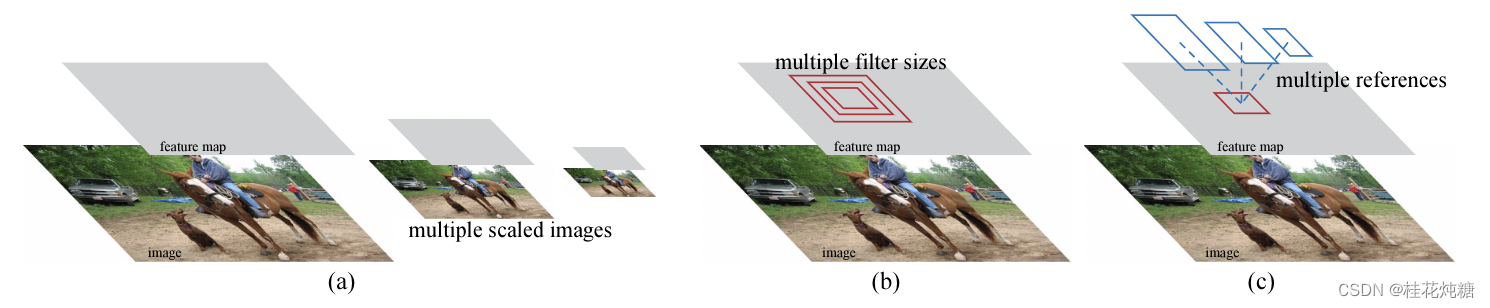
图1:解决多尺度和尺寸问题的不同方案。(a) 建立了图像金字塔和特征图,并在所有尺度上运行分类器。(b) 具有多个比例/大小的过滤器金字塔在要素图上运行。(c) 我们在回归函数中使用参考框的金字塔。
To unify RPNs with Fast RCNN [2] object detection networks, we propose a training scheme that alternates between fine-tuning for the region proposal task and then fine-tuning for object detection, while keeping the proposals fixed. This scheme converges quickly and produces a unified network with convolutional features that are shared between both tasks.
为了统一RPN和Fast R-CNN[5]目标检测网络,我们提出一种简单的训练方案,即保持候选框固定,微调区域建议和微调目标检测之间交替进行。这个方案收敛很快,最后形成可让两个任务共享卷积特征的标准网络。
We comprehensively evaluate our method on the PASCAL VOC detection benchmarks [11] where RPNs with Fast R-CNNs produce detection accuracy better than the strong baseline of Selective Search with Fast R-CNNs. Meanwhile, our method waives nearly all computational burdens of Selective Search at test-time—the effective running time for proposals is just 10 milliseconds. Using the expensive very deep models of [3], our detection method still has a frame rate of 5fps (including all steps) on a GPU,and thus is a practical object detection system interms of both speed and accuracy. We also reportresults on the MS COCO dataset [12] and investigate the improvements on PASCAL VOC using theCOCO data. Code has been made publicly available at https://github.com/shaoqingren/faster_rcnn(in MATLAB) and https://github.com/rbgirshick/py-faster-rcnn(in Python)
我们在PASCAL VOC检测基准上综合评估了我们的方法[11],其中使用快速R-CNN的RPN产生的检测精度比使用快速R-CNN的选择性搜索的强基准更好。同时,我们的方法几乎免除了选择性搜索的所有计算负担——提案的有效运行时间仅为10毫秒。使用[3]中昂贵的深度模型,我们的检测方法在GPU上仍具有5fps的帧速率(包括所有步骤),因此在速度和精度方面都是一个实用的目标检测系统。我们还报告了MS COCO数据集的结果[12],并使用COCO数据对PASCAL VOC的改进进行了研究。代码已公开leathttps://github.com/shaoqingren/faster_rcnn(在MATLAB中)andhttps://github.com/rbgirshick/py-faster-rcnn(在Python中)
A preliminary version of this manuscript was published previously [10]. Since then, the frameworks of RPN and Faster R-CNN have been adopted and generalized to other methods, such as 3D object detection[13], part-based detection [14], instance segmentation[15], and image captioning [16]. Our fast and effective object detection system has also been built in commercial systems such as at Pinterests [17], with user engagement improvements reported.In ILSVRC and COCO 2015 competitions, FasterR-CNN and RPN are the basis of several 1st-placeentries [18] in the tracks of ImageNet detection, ImageNet localization, COCO detection, and COCO segmentation. RPNs completely learn to propose regionsfrom data, and thus can easily benefit from deeperand more expressive features (such as the 101-layer residual nets adopted in [18]). Faster R-CNN and RPN are also used by several other leading entries in these competitions. These results suggest that our methodis not only a cost-efficient solution for practical usage,but also an effective way of improving object detection accuracy.
这份手稿的初步版本已在之前出版[10]。此后,RPN和Faster R-CNN的框架被采用并推广到其他方法,如3D对象检测[13]、基于部分的检测[14]、实例分割[15]和图像字幕[16]。我们的快速有效的目标检测系统也已内置于Pinterest[17]等商业系统,用户参与度有所提高。在ILSVRC和COCO 2015比赛中,FasterR CNN和RPN是ImageNet检测、ImageNet定位、COCO检测和COCO分割赛道中几个第一名的基础[18]。RPN完全可以从数据中学习提出区域,因此可以很容易地受益于深度和更具表现力的特征(如[18]中采用的101层残差网络)。更快的RCNN和RPN也被其他几项竞赛中的领先参赛作品所使用。这些结果表明,我们的方法不仅是一种实用的成本效益解决方案,也是提高目标检测精度的有效方法。
2.相关工作
Object Proposals.There is a large literature on objectproposal methods. Comprehensive surveys and comparisons of object proposal methods can be found in[19], [20], [21]. Widely used object proposal methods include those based on grouping super-pixels (e.g.,Selective Search [4], CPMC [22], MCG [23]) and those based on sliding windows (e.g., objectness in windows[24], EdgeBoxes [6]). Object proposal methods were adopted as external modules independent of the de-tectors (e.g., Selective Search [4] object detectors, R-CNN [5], and Fast R-CNN [2])
对象提案。有大量关于对象建议方法的文献。在[19]、[20]、[21]中可以找到对象提议方法的综合调查和比较。广泛使用的对象建议方法包括基于对超级像素进行分组的方法(例如,选择性搜索[4]、CPMC[22]、MCG[23])和基于滑动窗口的方法(如,窗口中的对象[24]、边缘框[6])。对象建议方法被采用为独立于检测器的外部模块(例如,选择性搜索[4]对象检测器、R-CNN[5]和快速R-CNN[2])
Deep Networks for Object Detection.The RCNN method [5] trains CNNs end-to-end to classify the proposal regions into object categories or background.RCNN mainly plays as a classifier, and it does not predict object bounds (except for refining by boundingbox regression). Its accuracy depends on the performance of the region proposal module (see comparisons in [20]). Several papers have proposed ways of using deep networks for predicting object boundingboxes [25], [9], [26], [27]. In the OverFeat method [9],a fully-connected layer is trained to predict the boxcoordinates for the localization task that assumes a single object. The fully-connected layer is then turned into a convolutional layer for detecting multiple class-specific objects. The MultiBox methods [26], [27] generate region proposals from a network whose last fully-connected layer simultaneously predicts multiple class-agnostic boxes, generalizing the “single-box” fashion of OverFeat. These class-agnostic boxes are used as proposals for R-CNN [5]. The MultiBox proposal network is applied on a single image crop or multiple large image crops (e.g., 224×224), in contrast to our fully convolutional scheme. MultiBox does not share features between the proposal and detection networks. We discuss OverFeat and MultiBox in more depth later in context with our method. Concurrent with our work, the DeepMask method [28] is developed for learning segmentation proposals
用于对象检测的深度网络。RCNN方法[5]对CNN进行端到端训练,以将提议区域分类为对象类别或背景。R-CNN主要充当分类器,它不预测对象边界(除了通过边界框回归进行细化)。其准确性取决于区域提案模块的性能(参见[20]中的比较)。几篇论文提出了使用深度网络预测对象边界框的方法[25],[9],[26],[27]。在OverFeat方法[9]中,训练一个完全连接的层来预测假设为单个对象的定位任务的框坐标。然后将完全连接的层翻转用于检测多个类特定对象。MultiBox方法[26]、[27]从网络中生成区域建议,该网络的最后一个连接层同时预测多个类别不可知的框,概括了OverFeat的“单一方框”方式。这些类别不可知的框被用作R-CNN的提案[5]。与我们的完全卷积方案相比,MultiBox方案网络应用于单个图像裁剪或多个大型图像裁剪(例如,224×224)。MultiBox在提案和检测网络之间不共享功能。我们稍后将结合我们的方法更深入地讨论OverFeat和MultiBox。与我们的工作同时开展,DeepMask方法[28]被开发用于学习分段建议
Shared computation of convolutions [9], [1], [29],[7], [2] has been attracting increasing attention for efficient, yet accurate, visual recognition. The OverFeat paper [9] computes convolutional features from an image pyramid for classification, localization, and detection. Adaptively-sized pooling (SPP) [1] on shared convolutional feature maps is developed for efficient region-based object detection [1], [30] and semantic segmentation [29]. Fast R-CNN [2] enables end-to-end detector training on shared convolutional features and shows compelling accuracy and speed
卷积的共享计算[9],[1],[29],[7],[2]因高效但准确的视觉识别而受到越来越多的关注。OverFeat[9]从图像金字塔中计算卷积特征,用于分类、定位和检测。基于共享卷积特征图的自适应大小池(SPP)[1]被开发用于高效的基于区域的对象检测[1]、[30]和语义分割[29]。Fast R-CNN[2]支持共享卷积特征的端到端检测器训练,并显示出令人信服的准确性和速度
3.Faster RCNN
Our object detection system, called Faster R-CNN, is composed of two modules. The first module is a deep fully convolutional network that proposes regions,and the second module is the Fast R-CNN detector [2]that uses the proposed regions. The entire system is a single, unified network for object detection (Figure 2).Using the recently popular terminology of neural networks with ‘attention’ [31] mechanisms, the RPN module tells the Fast R-CNN module where to look.In Section 3.1 we introduce the designs and propertiesof the network for region proposal. In Section 3.2 we develop algorithms for training both modules with features shared.
我们的目标检测系统称为Faster R-CNN,由两个模块组成。第一个模块是提出区域的深度卷积网络,第二个模块是使用提出区域的快速R-CNN检测器[2]。整个系统是用于对象检测的单一统一网络(图2)。使用最近流行的具有“注意力”机制的神经网络术语[31],RPN模块告诉Fast R-CNN模块该往哪里看。在第3.1节中,我们介绍了区域方案网络的设计和特性。在第3.2节中,我们开发了用于训练两个具有共享特征的模块的算法。
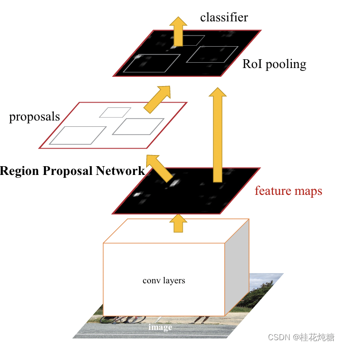
图2:Faster R-CNN是一个用于对象检测的单一统一网络。RPN模块充当这个统一网络的“注意力”
3.1区域建议网络
A Region Proposal Network (RPN) takes an image(of any size) as input and outputs a set of rectangular object proposals, each with an objectness score.We model this process with a fully convolutional network[7], which we describe in this section. Because our ulti-mate goal is to share computation with a Fast R-CNN object detection network [2], we assume that both nets share a common set of convolutional layers. In our experiments, we investigate the Zeiler and Fergus model[32] (ZF), which has 5 shareable convolutional layersand the Simonyan and Zisserman model [3] (VGG-16),which has 13 shareable convolutional layers.
区域建议网络(RPN)将一个图像(任意大小)作为输入,输出矩形目标建议框的集合,每个框有一个objectness得分。我们用全卷积网络[14]对这个过程构建模型,本章会详细描述。因为我们的最终目标是和Fast R-CNN目标检测网络[15]共享计算,所以假设这两个网络共享一系列卷积层。在实验中,我们详细研究Zeiler和Fergus的模型[23](ZF),它有5个可共享的卷积层,以及Simonyan和Zisserman的模型[19](VGG),它有13个可共享的卷积层。
To generate region proposals, we slide a small network over the convolutional feature map output by the last shared convolutional layer. This small network takes as input an n×n spatial window of the input convolutional feature map. Each sliding window is mapped to a lower-dimensional feature(256-d for ZF and 512-d for VGG, with ReLU [33] following). This feature is fed into two sibling fully-connected layers—a box-regression layer (reg) and a box-classification layer (cls). We use n= 3 in this paper, noting that the effective receptive field on theinput image is large (171 and 228 pixels for ZF andVGG, respectively). This mini-network is illustratedat a single position in Figure 3 (left). Note that because the mini-network operates in a sliding-window fashion, the fully-connected layers are shared across all spatial locations. This architecture is naturally im-plemented with an n×n convolutional layer followed by two sibling 1×1 convolutional layers (for reg and cls, respectively).
为了生成区域建议框,我们在最后一个共享的卷积层输出的卷积特征映射上滑动小网络,这个网络采用输入卷积特征映射的nxn的空间窗口作为输入。每个滑动窗口映射到一个低维向量上(对于ZF是256-d,对于VGG是512-d,ReLU紧随其后)。这个向量输出给两个同级的全连接的层——预测框回归层(reg)和预测框分类层(cls)。本文中n=3,注意图像的有效感受野很大(ZF是171像素,VGG是228像素)。图1(左)以这个小网络在某个位置的情况举了个例子。注意,由于小网络是滑动窗口的形式,所以全连接的层(nxn的)被所有空间位置共享(指所有位置用来计算内积的nxn的层参数相同)。这种结构实现为nxn的卷积层,后接两个同级的1x1的卷积层(分别对应reg和cls)
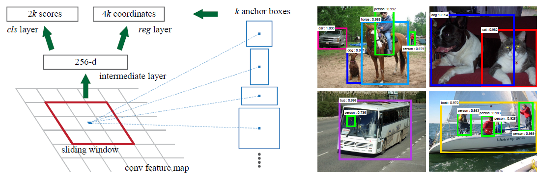
图3:左:区域建议网络(RPN)。右:用RPN建议框在PASCAL VOC 2007测试集上的检测实例。我们的方法可以在很大范围的尺度和长宽比中检测目标。
3.1.1 Anchors
At each sliding-window location, we simultaneously predict multiple region proposals, where the number of maximum possible proposals for each location is denoted as k. So the reg layer has 4k outputs encoding the coordinates of k boxes, and the cls layer outputs 2k scores that estimate probability of object or not object for each proposal. The k proposals are parameterized relative to k reference boxes, which we call anchors. An anchor is centered at the sliding window in question, and is associated with a scale and aspect ratio (Figure 3, left). By default we use 3 scales and 3 aspect ratios, yielding k= 9 anchors at each sliding position. For a convolutional feature map of a size W×H (typically∼2,400), there are WHk anchors in total
在每个滑动窗口位置,我们同时预测多个区域方案,其中每个位置的最大可能方框数表示为k。因此reg层有4k个输出来编码k个boxes的坐标,而cls层输出2k个得分来估计每个建议框是类别还是背景。(为简单起见,是用二类的softmax层实现的cls层,还可以用logistic回归来生成k个得分)k个建议框被称为相应的k个anchor的参数化,我们称之为锚框。锚定位于所讨论的滑动窗口的中心,并与尺度和长宽比相关联(图3,左侧)。默认情况下,我们使用3个尺度和3个长宽比,在每个滑动位置上产生k=9个锚框。对于尺寸为W×H的卷积特征图(通常∼2400),总共有W*H*k个锚框。
平移不变的anchor
An important property of our approach is that it is translation invariant, both in terms of the anchors and the functions that compute proposals relative to the anchors. If one translates an object in an image,the proposal should translate and the same function should be able to predict the proposal in either location. This translation-invariant property is guaranteed by our method. As a comparison, the MultiBox method [27] uses k-means to generate 800 anchors,which are not translation invariant. So MultiBox does not guarantee that the same proposal is generated if an object is translated.
我们的方法有一个重要特性,就是平移不变性,对anchor和对计算anchor相应的建议框的函数而言都是这样。如果平移了图像中的目标,建议框也应该平移,也应该能用同样的函数预测建议框。我们的方法保证了这种平移不变性。作为比较,MultiBox方法[20]用k-means生成800个anchor,但不具有平移不变性。因此,如果一个对象被平移,MultiBox不能保证生成相同的建议框。
The translation-invariant property also reduces the model size. MultiBox has a(4 + 1)×800-dimensional fully-connected output layer, whereas our method has a (4 + 2)×9-dimensional convolutional output layer in the case of k= 9 anchors. As a result, our output layer has 2.8×10^4 parameters (512×(4 + 2)×9 for VGG-16), two orders of magnitude fewer than MultiBox’s output layer that has 6.1×10^6 parameters (1536×(4 + 1)×800 for GoogleNet [34] in MultiBox[27]). If considering the feature projection layers, our proposal layers still have an order of magnitude fewer parameters than MultiBox6. We expect our method to have less risk of overfitting on small datasets, like PASCAL VOC.
平移不变属性还减小了模型大小。MultiBox具有(4+1)×800维全连接输出层,而我们的方法在k=9个锚的情况下具有(4+2)×9维卷积输出层。因此,我们的输出层有2.8×10^4个参数(VGG-16为512×(4+2)×9),比MultiBox的输出层少了两个数量级,后者有6.1×10^6个参数(MultiBox[27]中的GoogleNet[34]为1536×(4+1)×800)。如果考虑到特征投影层,我们的建议层的参数仍然比MultiBox6低一个数量级。我们预计我们的方法在小数据集上过度拟合的风险较小,如PASCAL VOC。
多尺度锚点作为回归参考
Our design of anchors presents a novel scheme for addressing multiple scales (and aspect ratios). As shown in Figure 1, there have been two popular ways for multiscale predictions. The first way is based on image/feature pyramids,e.g., in DPM [8] and CNN-based methods [9], [1], [2]. The images are resized at multiple scales, and feature maps (HOG [8] or deep convolutional features [9], [1], [2]) are computed for each scale (Figure 1(a)). This way is often useful but is time-consuming. The second way is to use sliding windows of multiple scales (and/or aspect ratios) on the feature maps. For example, in DPM [8], models of different aspect ratios are trained separately using different filter sizes (such as 5×7 and 7×5). If this wayis used to address multiple scales, it can be thought of as a “pyramid of filters” (Figure 1(b)). The second way is usually adopted jointly with the first way [8].
我们的锚框设计提出了一种解决多尺度(和长宽比)问题的新方案。如图1所示,有两种常用的多尺度预测方法。第一种方法是基于图像/特征金字塔,例如在DPM[8]和基于CNN的方法[9]、[1]、[2]中。在多个尺度上调整图像的大小,并针对每个尺度计算特征图(HOG[8]或深度卷积特征[9]、[1]、[2])(图1(a))。这种方法通常很有用,但很耗时。第二种方法是在特征图上使用多个比例(和/或长宽比)的滑动窗口。例如,在DPM[8]中,使用不同的滤波器大小(如5×7和7×5)分别训练不同长宽比的模型。如果这种方法用于处理多个尺度,可以将其视为“过滤器金字塔”(图1(b))。第二种方法通常与第一种方法联合使用[8]。
3.1.2 损失函数
For training RPNs, we assign a binary class label (of being an object or not) to each anchor. We assign a positive label to two kinds of anchors: (i) the anchor/anchors with the highest Intersection-over-Union (IoU) overlap with a ground-truth box,or(ii) an anchor that has an IoU overlap higher than 0.7 with any ground-truth box. Note that a single ground-truth box may assign positive labels to multiple anchors.Usually the second condition is sufficient to determine the positive samples; but we still adopt the first condition for the reason that in some rare cases these second condition may find no positive sample. We assign a negative label to a nonpositive anchor if its IoU ratio is lower than 0.3 for all ground-truth boxes.Anchors that are neither positive nor negative do not contribute to the training objective.
为了训练RPN,我们给每个anchor分配一个二进制的标签(是不是目标)。我们分配正标签给两类anchor:(i)与某个ground truth(GT)框有最高的IoU(Intersection-over-Union,交集并集之比)重叠的anchor(也许不到0.7),(ii)与任意GT框有大于0.7的IoU交叠的anchor。注意到一个GT框可能分配正标签给多个anchor。通常第二个条件足以确定正样本;但我们仍然采用第一种条件,因为在某些罕见情况下,第二种条件可能找不到正样本。我们分配负标签给与所有GT框的IoU比率都低于0.3的anchor。非正非负的anchor对训练目标没有任何作用。
With these definitions, we minimize an objectivefunction following the multi-task loss in Fast R-CNN[2]. Our loss function for an image is defined as
有了这些定义,我们遵循Fast R-CNN[5]中的多任务损失,最小化目标函数。我们对一个图像的损失函数定义为

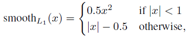
Here,i is the index of an anchor in a mini-batch and pi is the predicted probability of anchor i being an object. The ground-truth label pi∗ is 1 if the anchor is positive, and is 0 if the anchor is negative.ti is a vector representing the 4 parameterized coordinates of the predicted bounding box, and ti∗ is that of the ground-truth box associated with a positive anchor.The classification loss Lcls is log loss over two classes(object vs not object). For the regression loss, we use Lreg(ti,ti∗) =R(ti−ti*) where R is the robust loss function (smooth L1) defined in [2]. The term pi* Lreg means the regression loss is activated only for positive anchors (p∗i= 1) and is disabled otherwise (p∗i= 0).The outputs of the cls and reglayers consist of {pi} and {ti} respectively.
这里,i是一个mini-batch中anchor的索引,Pi是anchor i是目标的预测概率。如果anchor为正,GT标签Pi* 就是1,如果anchor为负,Pi* 就是0。ti是一个向量,表示预测框的4个参数化坐标,ti* 是与正anchor对应的GT框的坐标向量。分类损失Lcls是两个类别(目标vs.非目标)的对数损失
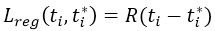
Pi* Lreg这一项意味着只有正anchor(Pi* =1)才有回归损失,其他情况就没有(Pi* =0)。cls层和reg层的输出分别由{pi}和{ti}组成
The two terms are normalized by Ncls and Nreg and weighted by a balancing parameter λ. In our current implementation (as in the released code), the cls term in Eqn.(1) is normalized by the mini-batchsize (i.e.,Ncls= 256) and theregterm is normalizedby the number of anchor locations (i.e.,Nreg∼2,400).By default we setλ= 10, and thus bothclsandregterms are roughly equally weighted. We showby experiments that the results are insensitive to thevalues ofλin a wide range (Table 9). We also notethat the normalization as above is not required andcould be simplified.For bounding box regression, we adopt the param-eterizations of the 4 coordinates following [5]:
这两项分别由Ncls和Nreg进行归一化以及一个平衡参数λ进行加权。在我们当前的实现中(如在发布的代码中),cls项通过最小批大小(即Ncls=256)归一化,reg项通过锚框位置的数量(即∼2,400)归一化。默认情况下,我们将λ设置为10,因此两个项的权重大致相等。我们通过实验表明,结果在很大范围内对λ值不敏感(表9)。我们还注意到,上述标准化是不需要的,可以简化。对于边界框回归,我们采用以下4个坐标的参数[5]

where x,y,w, and h denote the box’s center coordinates and its width and height. Variables x,xa, and x∗ are for the predicted box, anchor box, and ground-truth box respectively (likewise for y,w,h). This can be thought of as bounding-box regression from an anchor box to a nearby ground-truth box.
x,y,w,h指的是边界框中心的坐标、宽、高。变量x,xa,x*分别指预测框、anchor框、GT框(对y,w,h也是一样)。可以认为是从anchor框到附近的GT框的边界框回归。
Nevertheless, our method achieves bounding-box regression by a different manner from previous RoI-based (Region of Interest) methods [1], [2]. In [1],[2], bounding-box regression is performed on features pooled from arbitrarily sized RoIs, and the regression weights are shared by all region sizes. In our formulation, the features used for regression are of the same spatial size (3×3) on the feature maps. To account for varying sizes, a set of k bounding-box regressors are learned. Each regressor is responsible for one scale and one aspect ratio, and the k regressors do not share weights. As such, it is still possible to predict boxes of various sizes even though the features are of a fixed size/scale, thanks to the design of anchors.
然而,我们的方法通过与以前基于RoI(感兴趣区域)方法不同的方式实现了边界框回归[1],[2]。在[1]和[2]中,对从任意RoI中提取的特征执行边界框回归,回归权重由所有区域大小共享。在我们的公式中,用于回归的特征在特征图上具有相同的空间大小(3×3)。为了解释不同的大小,我们学习了一组K边界框回归。每个回归因子负责一个尺度和一个长宽比,而回归因子不共享权重。因此,由于锚框的设计,即使特征具有固定的尺寸/比例,仍然可以预测各种尺寸的边界框。
3.1.3 训练RPNs
The RPN can be trained end-to-end by back-propagation and stochastic gradient descent (SGD)[35]. We follow the “image-centric” sampling strategy from [2] to train this network. Each mini-batch arises from a single image that contains many positive and negative example anchors. It is possible to optimize for the loss functions of all anchors, but this will bias towards negative samples as they are dominate.Instead, we randomly sample 256 anchors in an image to compute the loss function of a mini-batch, where the sampled positive and negative anchors have a ratio of up to1:1. If there are fewer than 128 positive samples in an image, we pad the mini-batch with negative ones.
RPN通过反向传播和随机梯度下降(SGD)[12]进行端到端训练。我们遵循[5]中的“image-centric”采样策略训练这个网络。每个mini-batch来自一个包含许多正负anchor样本的图像。我们可以优化所有anchor的损失函数,但是这会偏向于负样本,因为它们是主要的。因此,我们随机地在一个图像中采样256个anchor,计算mini-batch的损失函数,其中采样的正负anchor的比例是1:1。如果一个图像中的正样本数小于128,我们就用负样本填补这个mini-batch。
We randomly initialize all new layers by drawing weights from a zero-mean Gaussian distribution with standard deviation 0.01. All other layers (i.e., the shared convolutional layers) are initialized by pre-training a model for ImageNet classification [36], as is standard practice [5]. We tune all layers of the ZF net, and conv3_1and up for the VGG net to conserve memory [2]. We use a learning rate of 0.001 for 60k mini-batches, and 0.0001 for the next 20k mini-batches on the PASCAL VOC dataset. We use a momentum of 0.9 and a weight decay of 0.0005 [37].Our implementation uses Caffe [38].
我们通过从零均值标准差为0.01的高斯分布中获取的权重来随机初始化所有新层(最后一个卷积层其后的层),所有其他层(即共享的卷积层)是通过对ImageNet分类[17]预训练的模型来初始化的,这也是标准惯例[6]。我们调整ZF网络的所有层,以及conv3_1,并为VGG网络做准备,以节约内存[5]。我们在PASCAL数据集上对于60k个mini-batch用的学习率为0.001,对于下一20k个mini-batch用的学习率是0.0001。动量是0.9,权重衰减为0.0005[11]。我们的实现使用了Caffe[10]。
3.2 RPN与Fast RCNN共享卷积特征
Thus far we have described how to train a network for region proposal generation, without considering the region-based object detection CNN that will utilize these proposals. For the detection network, we adopt Fast R-CNN [2]. Next we describe algorithms that learn a unified network composed of RPN and FastR-CNN with shared convolutional layers (Figure 2).
迄今为止,我们已经描述了如何为生成RPN训练网络,而没有考虑基于区域的目标检测CNN如何利用这些建议框。对于检测网络,我们采用Fast R-CNN[5],接下来我们描述学习由RPN和FastR CNN组成的具有共享卷积层的统一网络的算法(图2)。
Both RPN and Fast R-CNN, trained independently,will modify their convolutional layers in different ways. We therefore need to develop a technique that allows for sharing convolutional layers between the two networks, rather than learning two separate net-works. We discuss three ways for training networks with features shared:
RPN和Fast R-CNN都是独立训练的,要用不同方式修改它们的卷积层。因此我们需要开发一种允许两个网络间共享卷积层的技术,而不是分别学习两个网络。我们讨论了三种具有共享功能的培训网络的方法:
(i)Alternating training. In this solution, we first train RPN, and use the proposals to train Fast R-CNN.The network tuned by Fast R-CNN is then used to initialize RPN, and this process is iterated. This is the solution that is used in all experiments in this paper.
(i) 交替训练。在这个解决方案中,我们首先训练RPN,并使用这些建议来训练Fast R-CNN。然后使用Fast R-CNN调整的网络来初始化RPN,并且重复这个过程。这是本文所有实验中使用的解决方案。
(ii)Approximate joint training. In this solution, the RPN and Fast R-CNN networks are merged into one network during training as in Figure 2. In each SGD iteration, the forward pass generates region proposals which are treated just like fixed, pre-computed proposals when training a Fast R-CNN detector. The backward propagation takes place as usual, where for the shared layers the backward propagated signals from both the RPN loss and the Fast R-CNN loss are combined. This solution is easy to implement. But this solution ignores the derivative w.r.t. the proposal boxes’ coordinates that are also network responses,so is approximate. In our experiments, we have em-pirically found this solver produces close results, yet reduces the training time by about 25-50% comparing with alternating training. This solver is included in our released Python code.
(ii)近似联合训练。在该解决方案中,RPN和Fast R-CNN网络在训练期间被合并为一个网络,如图2所示。在一轮SGD的迭代中,前向传播传递生成的区域建议,这些建议在训练Fast R-CNN检测器时被视为固定的、预先计算的建议。反向传播照常进行,对于共享层来说,来自RPN的loss和Fast R-CNN的loss的反向传播信号被组合。此解决方案易于实施。但是该解决方案忽略了也会被网络响应的建议框的导数,因此是近似的。在我们的实验中,我们实验发现该解决方案产生了接近的结果,与交替训练相比,训练时间缩短了约25-50%。此解决方案包含在我们发布的Python代码中。
(iii)Non-approximate joint training. As discussed above, the bounding boxes predicted by RPN are also functions of the input. The RoI pooling layer[2] in Fast R-CNN accepts the convolutional features and also the predicted bounding boxes as input, so a theoretically valid backpropagation solver should also involve gradients w.r.t. the box coordinates. These gradients are ignored in the above approximate joint training. In a non-approximate joint training solution,we need an RoI pooling layer that is differentiable w.r.t. the box coordinates. This is a nontrivial problem and a solution can be given by an “RoI warping” layer as developed in [15], which is beyond the scope of this paper.
(iii)非近似联合训练。如上所述,RPN预测的边界框也是输入。Fast R-CNN中的RoI池化层[2]接受卷积特征以及预测的边界框作为输入,理论上有效的反向传播也应包括相对于框坐标的梯度。在上述近似联合训练中,忽略了这项。在非近似联合训练解决方案中,我们需要一个RoI池化层,该层可微分框坐标。这是一个非常重要的问题,可以通过[15]中开发的“RoI warping”层给出解决方案,这超出了本文的范围。
4-Step Alternating Training. In this paper, we adopt a pragmatic 4-step training algorithm to learn shared features via alternating optimization. In the first step,we train the RPN as described in Section 3.1.3. This network is initialized with an ImageNet-pre-trained model and fine-tuned end-to-end for the region proposal task. In the second step, we train a separate detection network by Fast R-CNN using the proposals generated by the step-1 RPN. This detection net-work is also initialized by the ImageNet-pre-trained model. At this point the two networks do not share convolutional layers. In the third step, we use the detector network to initialize RPN training, but we fix the shared convolutional layers and only fine-tunethe layers unique to RPN. Now the two networksshare convolutional layers. Finally, keeping the sharedconvolutional layers fixed, we fine-tune the uniquelayers of Fast R-CNN. As such, both networks sharethe same convolutional layers and form a unifiednetwork. A similar alternating training can be runfor more iterations, but we have observed negligibleimprovements.
4步交替训练。在本文中,我们采用了一种实用的四步训练算法,通过交替优化来学习共享特征。在第一步中,我们按照第3.1.3节所述训练RPN。该网络使用ImageNet预训练模型进行初始化,并针对区域建议框任务进行端到端微调。在第二步中,我们使用步骤1 RPN生成的建议,通过Fast R-CNN训练分离检测网络,该检测网络也由ImageNet预训练模型初始化。此时,两个网络不共享卷积层。在第三步中,我们使用检测器网络来初始化RPN训练,但是我们固定共享卷积层,仅微调RPN的特有层。现在这两个网络共享卷积层。最后,保持共享卷积层的固定,我们微调Fast R-CNN的特有层。因此,两个网络共享相同的卷积层并形成统一的网络。类似的交替训练可以运行更多的迭代,但我们观察到只有细微的提升
3.3 实现细节
We train and test both region proposal and object detection networks on images of a single scale [1], [2].We re-scale the images such that their shorter side is s= 600 pixels [2]. Multi-scale feature extraction(using an image pyramid) may improve accuracy but does not exhibit a good speed-accuracy trade-off [2].On the re-scaled images, the total stride for both ZFand VGG nets on the last convolutional layer is 16pixels, and thus is∼10 pixels on a typical PASCALimage before resizing (∼500×375). Even such a largestride provides good results, though accuracy may befurther improved with a smaller stride.
我们训练、测试区域建议和目标检测网络都是在单一尺度的图像上[7, 5]。我们缩放图像,让它们的短边s=600像素[5]。多尺度特征提取可能提高准确率但是不利于速度与准确率之间的权衡[5]。我们也注意到ZF和VGG网络,对缩放后的图像在最后一个卷积层的总步长为16像素,这样相当于一个典型的PASCAL缩放前的图像(~500x375)上大约10个像素。即使是这样大的步长也取得了好结果,尽管若步长小点准确率可能得到进一步提高。
For anchors, we use 3 scales with box areas of 128^2,256^2, and 512^2 pixels, and 3 aspect ratios of 1:1, 1:2,and 2:1. These hyper-parameters are not carefully chosen for a particular dataset, and we provide ablation experiments on their effects in the next section. As discussed, our solution does not need an image pyramid or filter pyramid to predict regions of multiple scales,saving considerable running time. Figure 3 (right)shows the capability of our method for a wide range of scales and aspect ratios. Table 1 shows the learned average proposal size for each anchor using the ZFnet. We note that our algorithm allows predictions that are larger than the underlying receptive field.Such predictions are not impossible—one may still roughly infer the extent of an object if only the middle of the object is visible
对于anchor,我们用3个简单的尺度,框面积为128x128,256x256,512x512,和3个简单的长宽比,1:1,1:2,2:1。这些超参数不是为特定的数据集精心选择的,我们在下一节中提供了关于其影响的消融实验。正如所讨论的,我们的解决方案不需要图像金字塔或滤波器金字塔来预测多尺度区域,节省了大量的运行时间。图3(右)显示了我们的方法在大范围尺度和长宽比下的能力。表1显示了使用ZFnet的每个锚的学习到的平均建议框大小。我们注意到,我们的算法允许比潜在的感受野更大的预测。这种预测并非不可能,如果只有物体的中间可见,人们仍然可以粗略地推断物体的范围。
下表是用ZF网络对每个anchor学到的平均建议框大小(s=600)。

The anchor boxes that cross image boundaries need to be handled with care. During training, we ignore all cross-boundary anchors so they do not contribute to the loss. For a typical 1000×600 image, there will be roughly 20000 (≈60×40×9) anchors in total. With the cross-boundary anchors ignored, thereare about 6000 anchors per image for training. If the boundary-crossing outliers are not ignored in training,they introduce large, difficult to correct error terms in the objective, and training does not converge. During testing, however, we still apply the fully convolutional RPN to the entire image. This may generate cross-boundary proposal boxes, which we clip to the image boundary.
需要小心处理跨越图像边界的锚定框。在训练中,我们忽略了所有跨越图像边界的anchor,这样它们不会对损失有影响。对于一个典型的1000x600的图像,差不多总共有20k(~60x40x9)anchor。忽略了跨越边界的anchor以后,每个图像只剩下6k个anchor需要训练了。如果跨越边界的异常值在训练时不忽略,就会带来又大又困难的修正误差项,训练也不会收敛。在测试时,我们还是应用全卷积的RPN到整个图像中,这可能生成跨越边界的建议框,我们将其裁剪到图像边缘位置。
Some RPN proposals highly overlap with each other. To reduce redundancy, we adopt non-maximum suppression (NMS) on the proposal regions based on their cls scores. We fix the IoU threshold for NMS at 0.7, which leaves us about 2000 proposal regions per image. As we will show, NMS does not harm the ultimate detection accuracy, but substantially reduces the number of proposals. After NMS, we use the top-N ranked proposal regions for detection. In the following, we train Fast R-CNN using 2000 RPN pro-posals, but evaluate different numbers of proposals at test-time.
有些RPN建议框和其他建议框大量重叠,为了减少冗余,我们基于建议区域的cls得分,对其采用非极大值抑制(non-maximum suppression, NMS)。我们固定对NMS的IoU阈值为0.7,这样每个图像只剩2k个建议区域。正如我们展示的,NMS不会影响最终的检测准确率,但是大幅地减少了建议框的数量。NMS之后,我们用建议区域中的top-N个来检测。在下文中,我们用2k个RPN建议框训练Fast R-CNN,但是在测试时会对不同数量的建议框进行评价。
4.实验
我们在PASCAL VOC2007检测基准[4]上综合评价我们的方法。此数据集包括20个目标类别,大约5k个trainval图像和5k个test图像。我们还对少数模型提供PASCAL VOC2012基准上的结果。对于ImageNet预训练网络,我们用“fast”版本的ZF网络[23],有5个卷积层和3个 fc层,公开的VGG-16 模型[19],有13 个卷积层和3 个fc层。我们主要评估检测的平均精度(mean Average Precision, mAP),因为这是对目标检测的实际度量标准(而不是侧重于目标建议框的代理度量)。
表1(上)显示了使用各种区域建议的方法训练和测试时Fast R-CNN的结果。这些结果使用的是ZF网络。对于选择性搜索(SS)[22],我们用“fast”模式生成了2k个左右的SS建议框。对于EdgeBoxes(EB)[24],我们把默认的EB设置调整为0.7IoU生成建议框。SS的mAP 为58.7%,EB的mAP 为58.6%。RPN与Fast R-CNN实现了有竞争力的结果,当使用300个建议框时的mAP就有59.9%(对于RPN,建议框数量,如300,是一个图像产生建议框的最大数量。RPN可能产生更少的建议框,这样建议框的平均数量也更少了)。使用RPN实现了一个比用SS或EB更快的检测系统,因为有共享的卷积计算;建议框较少,也减少了区域方面的fc消耗。接下来,我们考虑RPN的几种消融,然后展示使用非常深的网络时,建议框质量的提高。
表1 PASCAL VOC2007年测试集的检测结果(在VOC2007 trainval训练)。该检测器是Fast R-CNN与ZF,但使用各种建议框方法进行训练和测试。

消融试验。为了研究RPN作为建议框方法的表现,我们进行了多次消融研究。首先,我们展示了RPN和Fast R-CNN检测网络之间共享卷积层的影响。要做到这一点,我们在4步训练过程中的第二步后停下来。使用分离的网络时的结果稍微降低为58.7%(RPN+ ZF,非共享,表1)。我们观察到,这是因为在第三步中,当调整过的检测器特征用于微调RPN时,建议框质量得到提高。
接下来,我们理清了RPN在训练Fast R-CNN检测网络上的影响。为此,我们用2k个SS建议框和ZF网络训练了一个Fast R-CNN模型。我们固定这个检测器,通过改变测试时使用的建议区域,评估检测的mAP。在这些消融实验中,RPN不与检测器共享特征。
在测试时用300个RPN建议框替换SS,mAP为56.8%。mAP的损失是训练/测试建议框之间的不一致所致。该结果作为以下比较的基准。
有些奇怪的是,在测试时使用排名最高的100个建议框时,RPN仍然会取得有竞争力的结果(55.1%),表明这种高低排名的RPN建议框是准确的。另一种极端情况,使用排名最高的6k个RPN建议框(没有NMS)取得具有可比性的mAP(55.2%),这表明NMS不会降低检测mAP,反而可以减少误报。
接下来,我们通过在测试时分别移除RPN的cls和reg中的一个,研究它们输出的作用。当在测试时(因此没有用NMS/排名)移除cls层,我们从没有计算得分的区域随机抽取N个建议框。N =1k 时mAP几乎没有变化(55.8%),但当N=100则大大降低为44.6%。这表明,cls得分是排名最高的建议框准确的原因。
另一方面,当在测试时移除reg层(这样的建议框就直接是anchor框了),mAP下降到52.1%。这表明,高品质的建议框主要归功于回归后的位置。单是anchor框不足以精确检测。
我们还评估更强大的网络对RPN的建议框质量的作用。我们使用VGG-16训练RPN,并仍然使用上述SS+ZF检测器。mAP从56.8%(使用RPN+ZF)提高到59.2%(使用RPN+VGG)。这是一个满意的结果,因为它表明,RPN+VGG的建议框质量比RPN+ZF的更好。由于RPN+ZF的建议框是可与SS竞争的(训练和测试一致使用时都是58.7%),我们可以预期RPN+VGG比SS好。下面的实验证明这一假说。
VGG-16的检测准确率与运行时间。表2展示了VGG-16对建议框和检测的结果。使用RPN+VGG,Fast R-CNN对不共享特征的结果是68.5%,比SS基准略高。如上所示,这是因为由RPN+VGG产生的建议框比SS更准确。不像预先定义的SS,RPN是实时训练的,能从更好的网络获益。对特征共享的变型,结果是69.9%——比强大的SS基准更好,建议框几乎无损耗。我们跟随[5],在PASCAL VOC2007 trainval和2012 trainval的并集上进一步训练RPN,mAP是73.2%。跟[5]一样在VOC 2007 trainval+test和VOC2012 trainval的并集上训练时,我们的方法在PASCAL VOC 2012测试集上(表3)有70.4%的mAP。
表2:在PASCAL VOC 2007测试集上的检测结果,检测器是Fast R-CNN和VGG16。训练数据:“07”:VOC2007 trainval,“07+12”:VOC 2007 trainval和VOC 2012 trainval的并集。对RPN,用于Fast R-CNN训练时的建议框是2k。这在[5]中有报告;利用本文所提供的仓库(repository),这个数字更高(68.0±0.3在6次运行中)。
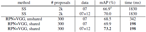
表3:PASCAL VOC 2012测试集检测结果。检测器是Fast R-CNN和VGG16。训练数据:“07”:VOC 2007 trainval,“07++12”: VOC 2007 trainval+test和VOC 2012 trainval的并集。对RPN,用于Fast R-CNN训练时的建议框是2k。
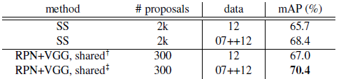
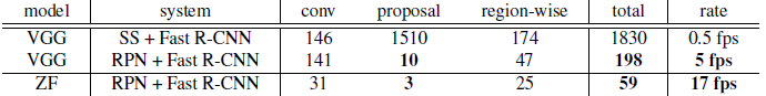
表4中我们总结整个目标检测系统的运行时间。SS需要1~2秒,取决于图像内容(平均1.51s),采用VGG-16的Fast R-CNN在2k个SS建议框上需要320ms(若是用了SVD在fc层的话只用223ms[5])。我们采用VGG-16的系统生成建议框和检测一共只需要198ms。卷积层共享时,RPN只用10ms来计算附加的几层。由于建议框较少(300),我们的区域计算花费也很低。我们的系统采用ZF网络时的帧率为17fps。
表4: K40 GPU上的用时(ms),除了SS建议框是在CPU中进行评价的。“区域方面”包括NMS,pooling,fc和softmax。请参阅我们发布的代码运行时间的分析。
IoU召回率的分析。接下来,我们计算建议框与GT框在不同的IoU比例时的召回率。值得注意的是,该IoU召回率度量标准与最终的检测准确率只是松散[9, 8, 1]相关的。更适合用这个度量标准来诊断建议框方法,而不是对其进行评估。
在图2中,我们展示使用300,1k,和2k个建议框的结果。我们将SS和EB作比较,并且这N个建议框是基于用这些方法生成的按置信度排名的前N个。该图显示,当建议框数量由2k下降到300时,RPN方法的表现很好。这就解释了使用少到300个建议框时,为什么RPN有良好的最终检测mAP。正如我们前面分析的,这个属性主要是归因于RPN的cls项。当建议框变少时,SS和EB的召回率下降的速度快于RPN。
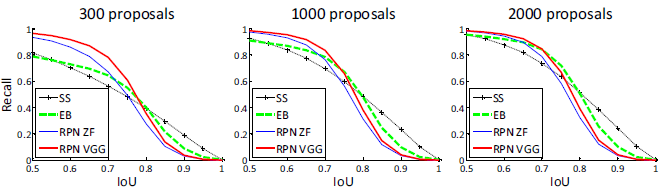
图2:PASCAL VOC 2007测试集上的召回率 vs. IoU重叠率
**单级的检测vs. 两级的建议框+检测。**OverFeat论文[18]提出在卷积特征映射的滑动窗口上使用回归和分类的检测方法。OverFeat是一个单级的,类特定的检测流程,我们的是一个两级的,由类无关的建议框方法和类特定的检测组成的级联方法。在OverFeat中,区域方面的特征来自一个滑动窗口,对应一个尺度金字塔的一个长宽比。这些特征被用于同时确定物体的位置和类别。在RPN中,特征都来自相对于anchor的方形(3*3)滑动窗口和预测建议框,是不同的尺度和长宽比。虽然这两种方法都使用滑动窗口,区域建议任务只是RPN + Fast R-CNN的第一级——检测器致力于改进建议框。在我们级联方法的第二级,区域一级的特征自适应地从建议框进行pooling[7, 5],更如实地覆盖区域的特征。我们相信这些特征带来更准确的检测。
为了比较单级和两级系统,我们通过单级的Fast R-CNN模拟OverFeat系统(因而也规避实现细节的其他差异)。在这个系统中,“建议框”是稠密滑动的,有3个尺度(128,256,512)和3个长宽比(1:1,1:2,2:1)。Fast R-CNN被训练来从这些滑动窗口预测特定类的得分和回归盒的位置。由于OverFeat系统采用多尺度的特征,我们也用由5个尺度中提取的卷积特征来评价。我们使用[7,5]中一样的5个尺度。
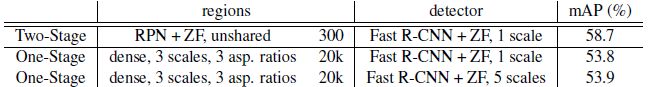
表5比较了两级系统和两个单级系统的变体。使用ZF模型,单级系统具有53.9%的mAP。这比两级系统(58.7%)低4.8%。这个实验证明级联区域建议方法和目标检测的有效性。类似的观察报告在[5,13]中,在两篇论文中用滑动窗口取代SS区域建议都导致了约6%的下降。我们还注意到,单级系统比较慢,因为它有相当多的建议框要处理。
表5:单级检测vs.两级建议+检测。检测结果都是在PASCAL VOC2007测试集使用ZF模型和Fast R-CNN。RPN使用非共享的特征。
5.总结
我们对高效和准确的区域建议的生成提出了区域建议建议网络(RPN)。通过与其后的检测网络共享卷积特征,区域建议的步骤几乎是无损耗的。我们的方法使一个一致的,基于深度学习的目标检测系统以5-17 fps的速度运行。学到的RPN也改善了区域建议的质量,进而改善整个目标检测的准确性。
表6:Fast R-CNN检测器和VGG16在PASCAL VOC 2007测试集的结果。对于RPN,Fast R-CNN训练时的建议框是2k个。RPN*表示非共享特征的版本。*
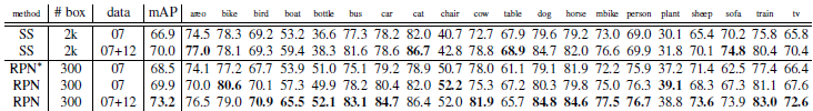
表7:Fast R-CNN检测器和VGG16在PASCAL VOC 2012测试集的结果。对于RPN,Fast R-CNN训练时的建议框是2k个。
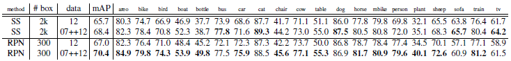
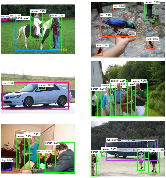
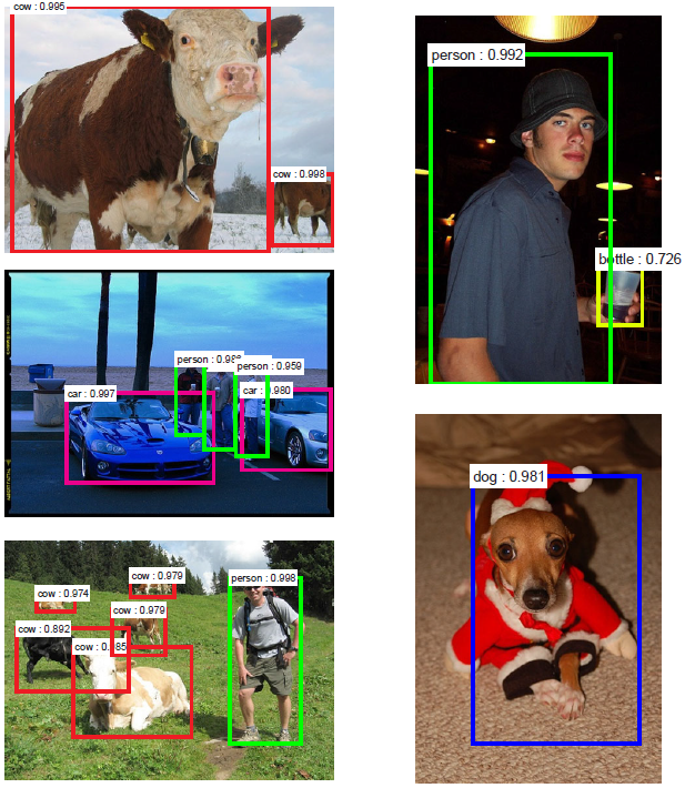
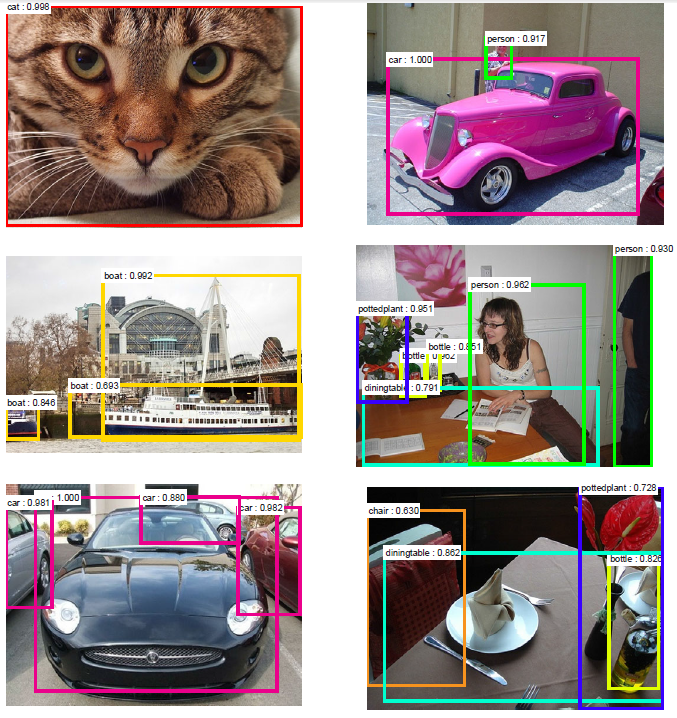
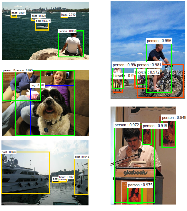
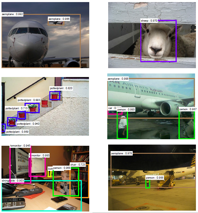
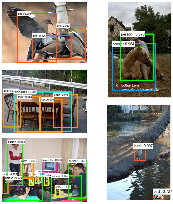
图3:对最终的检测结果使用具有共享特征的RPN + FastR-CNN在PASCAL VOC 2007测试集上的例子。模型是VGG16,训练数据是07 + 12trainval。我们的方法检测的对象具有范围广泛的尺度和长宽比。每个输出框与一个类别标签和一个范围在[0,1]的softmax得分相关联。显示这些图像的得分阈值是0.6。取得这些结果的运行时间是每幅图像198ms,包括所有步骤。