Reinforcement Learning with Code
This note records how the author begin to learn RL. Both theoretical understanding and code practice are presented. Many material are referenced such as ZhaoShiyu’s Mathematical Foundation of Reinforcement Learning, .
文章目录
- Reinforcement Learning with Code
- Chapter 9. Policy Gradient Methods
- 9.1 Basic idea of policy gradient
- 9.2 Metrics to define optimal policies
- 9.3 Gradients of the metrics
- 9.4 Policy gradient by Monte Carlo estimation: REINFORCE
- Reference
Chapter 9. Policy Gradient Methods
The idea of function approximation can be applied to represent not only state/action values but also policies. Up to now in this book, policies have been represented by tables: the action probabilities of all states are stored in a table π ( a ∣ s ) \pi(a|s) π(a∣s), each entry of which is indexed by a state and an action. In this chapter, we show that polices can be represented by parameterized functions denoted as π ( a ∣ s , θ ) \pi(a|s,\theta) π(a∣s,θ), where θ ∈ R m \theta\in\mathbb{R}^m θ∈Rm is a parameter vector. The function representation is also sometimes written as π ( a , s , θ ) , π θ ( a ∣ s ) , \textcolor{blue}{\pi(a,s,\theta)},\textcolor{blue}{\pi_\theta(a|s)}, π(a,s,θ),πθ(a∣s), or π θ ( a , s ) \textcolor{blue}{\pi_\theta(a,s)} πθ(a,s).
When policies are represented as a function, optimal policies can be found by optimizing certain scalar metrics. Such kind of method is called policy gradient.
9.1 Basic idea of policy gradient
How to define optimal policies? When represented as a table, a policy π \pi π is defined as optimal if it can maximize every state value. When represented by a function, a policy π \pi π is fully determined by θ \theta θ together with the function strcuture. The policy is defined as optimal if it can maximize certain scalar metrics, which we will introduce later.
How to update policies? When represented as a table, a plicy π \pi π can be updated by directly changing the entries in the table. However, when represented by a parameterized function, a policy π \pi π cannot be updated in this way anymore. Instead, it can only be improved by updating the parameter θ \theta θ. We can use gradient-based method to optimize some metrics to update the parameter θ \theta θ.
9.2 Metrics to define optimal policies
The first metric is the average state value or simply called average value. Let
v π = [ ⋯ , v π ( s ) , ⋯ ] T ∈ R ∣ S ∣ d π = [ ⋯ , d π ( s ) , ⋯ ] T ∈ R ∣ S ∣ v_\pi = [\cdots, v_\pi(s), \cdots]^T \in \mathbb{R}^{|\mathcal{S}|} \\ d_\pi = [\cdots, d_\pi(s), \cdots]^T \in \mathbb{R}^{|\mathcal{S}|} vπ=[⋯,vπ(s),⋯]T∈R∣S∣dπ=[⋯,dπ(s),⋯]T∈R∣S∣
be the vector of state values and a vector of distribution of state value, respectively. Here, d π ( s ) ≥ 0 d_\pi(s)\ge 0 dπ(s)≥0 is the weight for state s s s and satisfies ∑ s d π ( s ) = 1 \sum_s d_\pi(s)=1 ∑sdπ(s)=1. The metric of average value is defined as
v ˉ π ≜ d π T v π = ∑ s d π ( s ) v π ( s ) = E [ v π ( S ) ] \begin{aligned} \textcolor{red}{\bar{v}_\pi} & \textcolor{red}{\triangleq d_\pi^T v_\pi} \\ & \textcolor{red}{= \sum_s d_\pi(s)v_\pi(s)} \\ & \textcolor{red}{= \mathbb{E}[v_\pi(S)]} \end{aligned} vˉπ≜dπTvπ=s∑dπ(s)vπ(s)=E[vπ(S)]
where S ∼ d π S \sim d_\pi S∼dπ. As its name suggests, v ˉ π \bar{v}_\pi vˉπ is simply a weighted average of the state values. The distribution d π ( s ) d_\pi(s) dπ(s) statisfies stationary distribution by sovling the equation
d π T P π = d π T d^T_\pi P_\pi = d^T_\pi dπTPπ=dπT
where P π P_\pi Pπ is the state transition probability matrix.
The second metrics is the average one-step rewrad or simply called average reward. Let
r π = [ ⋯ , r π ( s ) , ⋯ ] T ∈ R ∣ S ∣ r_\pi = [\cdots, r_\pi(s),\cdots]^T \in \mathbb{R}^{|\mathcal{S}|} rπ=[⋯,rπ(s),⋯]T∈R∣S∣
be the vector of one-step immediate rewards. Here
r π ( s ) = ∑ a π ( a ∣ s ) r ( s , a ) r_\pi(s) = \sum_a \pi(a|s)r(s,a) rπ(s)=a∑π(a∣s)r(s,a)
is the average of the one-step immediate reward that can be obtained starting from state s s s, and r ( s , a ) = E [ R ∣ s , a ] = ∑ r r p ( r ∣ s , a ) r(s,a)=\mathbb{E}[R|s,a]=\sum_r r p(r|s,a) r(s,a)=E[R∣s,a]=∑rrp(r∣s,a) is the average of the one-step immediate reward that can be obtained after taking action a a a at state s s s. Then the metric is defined as
r ˉ π ≜ d π T r π = ∑ s d π ( s ) ∑ a π ( a ∣ s ) ∑ r r p ( r ∣ s , a ) = ∑ s d π ( s ) ∑ a π ( a ∣ s ) r ( s , a ) = ∑ s d π ( s ) r π ( s ) = E [ r π ( S ) ] \begin{aligned} \textcolor{red}{\bar{r}_\pi} & \textcolor{red}{\triangleq d_\pi^T r_\pi} \\ & \textcolor{red}{= \sum_s d_\pi(s)\sum_a \pi(a|s) \sum_r r p(r|s,a) } \\ & \textcolor{red}{= \sum_s d_\pi(s)\sum_a \pi(a|s)r(s,a) } \\ & \textcolor{red}{= \sum_s d_\pi(s)r_\pi(s)} \\ & \textcolor{red}{= \mathbb{E}[r_\pi(S)]} \end{aligned} rˉπ≜dπTrπ=s∑dπ(s)a∑π(a∣s)r∑rp(r∣s,a)=s∑dπ(s)a∑π(a∣s)r(s,a)=s∑dπ(s)rπ(s)=E[rπ(S)]
where S ∼ d π S\sim d_\pi S∼dπ. As its name suggests, r ˉ π \bar{r}_\pi rˉπ is simply a weighted average of the one-step immediate rewards.
The third metric is the state value of a specific starting state v π ( s 0 ) v_\pi(s_0) vπ(s0). For some tasks, we can only start from a specific state s 0 s_0 s0. In this case, we only care about the long-term return starting from s 0 s_0 s0. This metric can also be viewed as a weighted average of the state values.
v π ( s 0 ) = ∑ s ∈ S d 0 ( s ) v π ( s ) \textcolor{red}{v_\pi(s_0) = \sum_{s\in\mathcal{S}} d_0(s) v_\pi(s)} vπ(s0)=s∈S∑d0(s)vπ(s)
where d 0 ( s = s 0 ) = 1 , d 0 ( s ≠ s 0 ) = 0 d_0(s=s_0)=1, d_0(s\ne s_0)=0 d0(s=s0)=1,d0(s=s0)=0.
We aim to search different value of parameter θ \theta θ to maximize these metrics.
9.3 Gradients of the metrics
Theorem 9.1 (Policy gradient theorem). The gradient of the average reward r ˉ π \bar{r}_\pi rˉπ metric is
∇ θ r ˉ π ( θ ) ≃ ∑ s d π ( s ) ∑ a ∇ θ π ( a ∣ s , θ ) q π ( s , a ) \textcolor{blue}{\nabla_\theta \bar{r}_\pi(\theta) \simeq \sum_s d_\pi(s)\sum_a \nabla_\theta \pi(a|s,\theta) q_\pi(s,a)} ∇θrˉπ(θ)≃s∑dπ(s)a∑∇θπ(a∣s,θ)qπ(s,a)
where ∇ θ π \nabla_\theta \pi ∇θπ is the gradient of π \pi π with respect to θ \theta θ. Here ≃ \simeq ≃ refers to either strict equality or approximated equality. In particular, it is a strict equation in the undiscounted case where γ = 1 \gamma=1 γ=1 and an approximated equation in the discounted case where 0 < γ < 1 0<\gamma<1 0<γ<1. The approximation is more accurate in the discounted case when γ \gamma γ is closer to 1 1 1. Moreover, the equation has a more compact and useful form expressed in terms of expectation:
∇ θ r ˉ π ( θ ) ≃ E [ ∇ θ ln π ( A ∣ S , θ ) q π ( S , A ) ] \textcolor{red}{\nabla_\theta \bar{r}_\pi(\theta) \simeq \mathbb{E} [\nabla_\theta \ln \pi(A|S,\theta)q_\pi(S,A)]} ∇θrˉπ(θ)≃E[∇θlnπ(A∣S,θ)qπ(S,A)]
where ln \ln ln is the natural logarithm and S ∼ d π , A ∼ π ( S ) S\sim d_\pi, A\sim \pi(S) S∼dπ,A∼π(S).
Why the two equations mentioned above is equivalent? Here is the derivation process
∇ θ r ˉ π ( θ ) ≃ ∑ s d π ( s ) ∑ a ∇ θ π ( a ∣ s , θ ) q π ( s , a ) = E [ ∑ a ∇ θ π ( a ∣ S , θ ) q π ( S , a ) ] \begin{aligned} \nabla_\theta \bar{r}_\pi(\theta) & \simeq \sum_s d_\pi(s)\sum_a \nabla_\theta \pi(a|s,\theta) q_\pi(s,a) \\ & = \mathbb{E}\Big[ \sum_a \nabla_\theta \pi(a|S,\theta) q_\pi(S,a) \Big] \end{aligned} ∇θrˉπ(θ)≃s∑dπ(s)a∑∇θπ(a∣s,θ)qπ(s,a)=E[a∑∇θπ(a∣S,θ)qπ(S,a)]
where S ∼ d π ( s ) S \sim d_\pi(s) S∼dπ(s). Furthermore, consider the function ln π \ln\pi lnπ where ln \ln ln is the natural algorithm.
∇ θ ln π ( a ∣ s , θ ) = ∇ θ π ( a ∣ s , θ ) π ( a ∣ s , θ ) → ∇ θ π ( a ∣ s , θ ) = π ( a ∣ s , θ ) ∇ θ ln π ( a ∣ s , θ ) \begin{aligned} \nabla_\theta \ln \pi (a|s,\theta) & = \frac{\nabla_\theta \pi(a|s,\theta)}{\pi(a|s,\theta)} \\ \to \nabla_\theta \pi(a|s,\theta) &= \pi(a|s,\theta) \nabla_\theta \ln \pi (a|s,\theta) \end{aligned} ∇θlnπ(a∣s,θ)→∇θπ(a∣s,θ)=π(a∣s,θ)∇θπ(a∣s,θ)=π(a∣s,θ)∇θlnπ(a∣s,θ)
By substituting
∇ θ r ˉ π ( θ ) = E [ ∑ a ∇ θ π ( a ∣ S , θ ) q π ( S , a ) ] = E [ ∑ a π ( a ∣ S , θ ) ∇ θ ln π ( a ∣ S , θ ) q π ( S , a ) ] = E [ ∇ θ ln π ( A ∣ S , θ ) q π ( S , A ) ] \begin{aligned} \nabla_\theta \bar{r}_\pi(\theta) & = \mathbb{E}\Big[ \sum_a \nabla_\theta \pi(a|S,\theta) q_\pi(S,a) \Big] \\ & = \mathbb{E}\Big[ \sum_a \pi(a|S,\theta) \nabla_\theta \ln \pi (a|S,\theta) q_\pi(S,a) \Big] \\ & = \mathbb{E}\Big[ \nabla_\theta \ln \pi (A|S,\theta) q_\pi(S,A) \Big] \end{aligned} ∇θrˉπ(θ)=E[a∑∇θπ(a∣S,θ)qπ(S,a)]=E[a∑π(a∣S,θ)∇θlnπ(a∣S,θ)qπ(S,a)]=E[∇θlnπ(A∣S,θ)qπ(S,A)]
where A ∼ π ( s , θ ) A \sim \pi(s,\theta) A∼π(s,θ).
Next we will show the metrics average one-step reward r ˉ π \bar{r}_\pi rˉπ and average state value v ˉ π \bar{v}_\pi vˉπ is equivalent. When discounted rate γ ∈ [ 0 , 1 ) \gamma\in[0,1) γ∈[0,1) is given, that
r ˉ π = ( 1 − γ ) v ˉ π \textcolor{blue}{\bar{r}_\pi = (1-\gamma)\bar{v}_\pi} rˉπ=(1−γ)vˉπ
Proof, note that v ˉ π ( θ ) = d π T v π \bar{v}_\pi(\theta)=d^T_\pi v_\pi vˉπ(θ)=dπTvπ and r ˉ = d π T r π \bar{r}=d^T_\pi r_\pi rˉ=dπTrπ, where v π v_\pi vπ and r π r_\pi rπ statisfy the Bellman equation v π = r π + γ P π v π v_\pi=r_\pi + \gamma P_\pi v_\pi vπ=rπ+γPπvπ. Then multiplying d π T d_\pi^T dπT on the both left sides of the Bellman equation gives
v ˉ π = r ˉ π + γ d π T P π v π = r ˉ π + γ d π T v π = r ˉ π + γ v ˉ π \bar{v}_\pi = \bar{r}_\pi + \gamma d^T_\pi P_\pi v_\pi = \bar{r}_\pi + \gamma d^T_\pi v_\pi = \bar{r}_\pi + \gamma \bar{v}_\pi vˉπ=rˉπ+γdπTPπvπ=rˉπ+γdπTvπ=rˉπ+γvˉπ
which implies r ˉ π = ( 1 − γ ) v ˉ π \bar{r}_\pi = (1-\gamma)\bar{v}_\pi rˉπ=(1−γ)vˉπ.
Theorem 9.2 (Gradient of v π ( s 0 ) v_\pi(s_0) vπ(s0) in the discounted case). In the discounted case where γ ∈ [ 0 , 1 ) \gamma \in [0,1) γ∈[0,1), the gradients of v π ( s 0 ) v_\pi(s_0) vπ(s0) is
∇ θ v π ( s 0 ) = E [ ∇ θ ln π ( A ∣ S , θ ) q π ( S , A ) ] \nabla_\theta v_\pi(s_0) = \mathbb{E}[\nabla_\theta \ln \pi(A|S, \theta)q_\pi(S,A)] ∇θvπ(s0)=E[∇θlnπ(A∣S,θ)qπ(S,A)]
where S ∼ ρ π S \sim \rho_\pi S∼ρπ and A ∼ π ( s , θ ) A \sim \pi(s,\theta) A∼π(s,θ). Here, the state distribution ρ π \rho_\pi ρπ is
ρ π ( s ) = Pr π ( s ∣ s 0 ) = ∑ k = 0 γ k Pr ( s 0 → s , k , π ) = [ ( I n − γ P π ) − 1 ] s 0 , s \rho_\pi(s) = \Pr_\pi (s|s_0) = \sum_{k=0} \gamma^k \Pr (s_0\to s, k, \pi) = [(I_n - \gamma P_\pi)^{-1}]_{s_0,s} ρπ(s)=πPr(s∣s0)=k=0∑γkPr(s0→s,k,π)=[(In−γPπ)−1]s0,s
which is the discounted total probability transiting from s 0 s_0 s0 to s s s under policy π \pi π.
Theorem 9.3 (Gradient of v ˉ π \bar{v}_\pi vˉπ and r ˉ π \bar{r}_\pi rˉπ in the discounted case). In the discounted case where γ ∈ [ 0 , 1 ) \gamma \in [0,1) γ∈[0,1), the gradients of v ˉ π \bar{v}_\pi vˉπ and r ˉ π \bar{r}_\pi rˉπ are, respectively,
∇ θ v ˉ π ≈ 1 1 − γ ∑ s d π ( s ) ∑ a ∇ θ π ( a ∣ s , θ ) q π ( s , a ) ∇ θ r ˉ π ≈ ∑ s d π ( s ) ∑ a ∇ θ π ( a ∣ s , θ ) q π ( s , a ) \begin{aligned} \nabla_\theta \bar{v}_\pi & \approx \frac{1}{1-\gamma} \sum_s d_\pi(s) \sum_a \nabla_\theta \pi(a|s,\theta) q_\pi(s,a) \\ \nabla_\theta \bar{r}_\pi & \approx \sum_s d_\pi(s) \sum_a \nabla_\theta \pi(a|s,\theta) q_\pi(s,a) \end{aligned} ∇θvˉπ∇θrˉπ≈1−γ1s∑dπ(s)a∑∇θπ(a∣s,θ)qπ(s,a)≈s∑dπ(s)a∑∇θπ(a∣s,θ)qπ(s,a)
where the approximations are more accurate when γ \gamma γ is closer to 1 1 1.
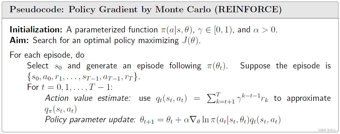
9.4 Policy gradient by Monte Carlo estimation: REINFORCE
Consider J ( θ ) = r ˉ π ( θ ) J(\theta) = \bar{r}_\pi(\theta) J(θ)=rˉπ(θ) or v π ( s 0 ) v_\pi(s_0) vπ(s0). The gradient-ascent algorithm maximizing J ( θ ) J(\theta) J(θ) is
θ t + 1 = θ t + α ∇ θ J ( θ ) = θ t + α E [ ∇ θ ln π ( A ∣ S , θ t ) q π ( S , A ) ] \begin{aligned} \theta_{t+1} & = \theta_t + \alpha \nabla_\theta J(\theta) \\ & = \theta_t + \alpha \mathbb{E}[\nabla_\theta \ln\pi(A|S,\theta_t) q_\pi(S,A)] \end{aligned} θt+1=θt+α∇θJ(θ)=θt+αE[∇θlnπ(A∣S,θt)qπ(S,A)]
where α > 0 \alpha>0 α>0 is a constant learning rate. Since the expected value on the right-hand side is unknown, we can replace the expected value with a sample (the idea of stochastic gradient). Then we have
θ t + 1 = θ t + α ∇ θ ln π ( a t ∣ s t , θ t ) q π ( s t , a t ) \theta_{t+1} = \theta_t + \alpha \nabla_\theta \ln\pi(a_t|s_t,\theta_t) q_\pi(s_t,a_t) θt+1=θt+α∇θlnπ(at∣st,θt)qπ(st,at)
However this cannot be implemented because q π ( s t , a t ) q_\pi(s_t,a_t) qπ(st,at) is the true value we can’t obtain. Hence, we use q t ( s t , a t ) q_t(s_t,a_t) qt(st,at) to estimate the true action value q π ( s t , a t ) q_\pi(s_t,a_t) qπ(st,at).
θ t + 1 = θ t + α ∇ θ ln π ( a t ∣ s t , θ t ) q t ( s t , a t ) \theta_{t+1} = \theta_t + \alpha \nabla_\theta \ln\pi(a_t|s_t,\theta_t) q_t(s_t,a_t) θt+1=θt+α∇θlnπ(at∣st,θt)qt(st,at)
If q π ( s t , a t ) q_\pi(s_t,a_t) qπ(st,at) is approximated by Monte Carlo estimation,
q π ( s t , a t ) ≜ E [ G t ∣ S t = s t , A t = a t ] ≈ 1 n ∑ i = 1 n g ( i ) ( s t , a t ) \begin{aligned} q_\pi(s_t,a_t) & \triangleq \mathbb{E}[G_t|S_t=s_t, A_t=a_t] \\ & \textcolor{blue}{\approx \frac{1}{n} \sum_{i=1}^n g^{(i)}(s_t,a_t)} \\ \end{aligned} qπ(st,at)≜E[Gt∣St=st,At=at]≈n1i=1∑ng(i)(st,at)
with stochastic approximation we don’t need to collect n n n episode start from ( s t , a t ) (s_t,a_t) (st,at) to approximate q π ( s t , a t ) q_\pi(s_t,a_t) qπ(st,at), we just need a discounted return starting from ( s t , a t ) (s_t,a_t) (st,at)
q π ( s t , a t ) ≈ q t ( a t , a t ) = ∑ k = t + 1 T γ k − t − 1 r k q_\pi(s_t,a_t) \approx q_t(a_t,a_t) = \sum_{k=t+1}^T \gamma^{k-t-1}r_k qπ(st,at)≈qt(at,at)=k=t+1∑Tγk−t−1rk
The algorithm is called REINFORCE.
Pseudocode:
Reference
赵世钰老师的课程